Introducing Packed BERT for 2x Training Speed-up in Natural Language Processing

By using a new packing algorithm, we have sped up Natural Language Processing by more than 2 times while training BERT-Large. Our new packing technique removes padding, enabling significantly more efficient computation.

We suspect this could also be applied to genomics and protein folding models and other models with skewed length distributions to make a much broader impact in different industries and applications.

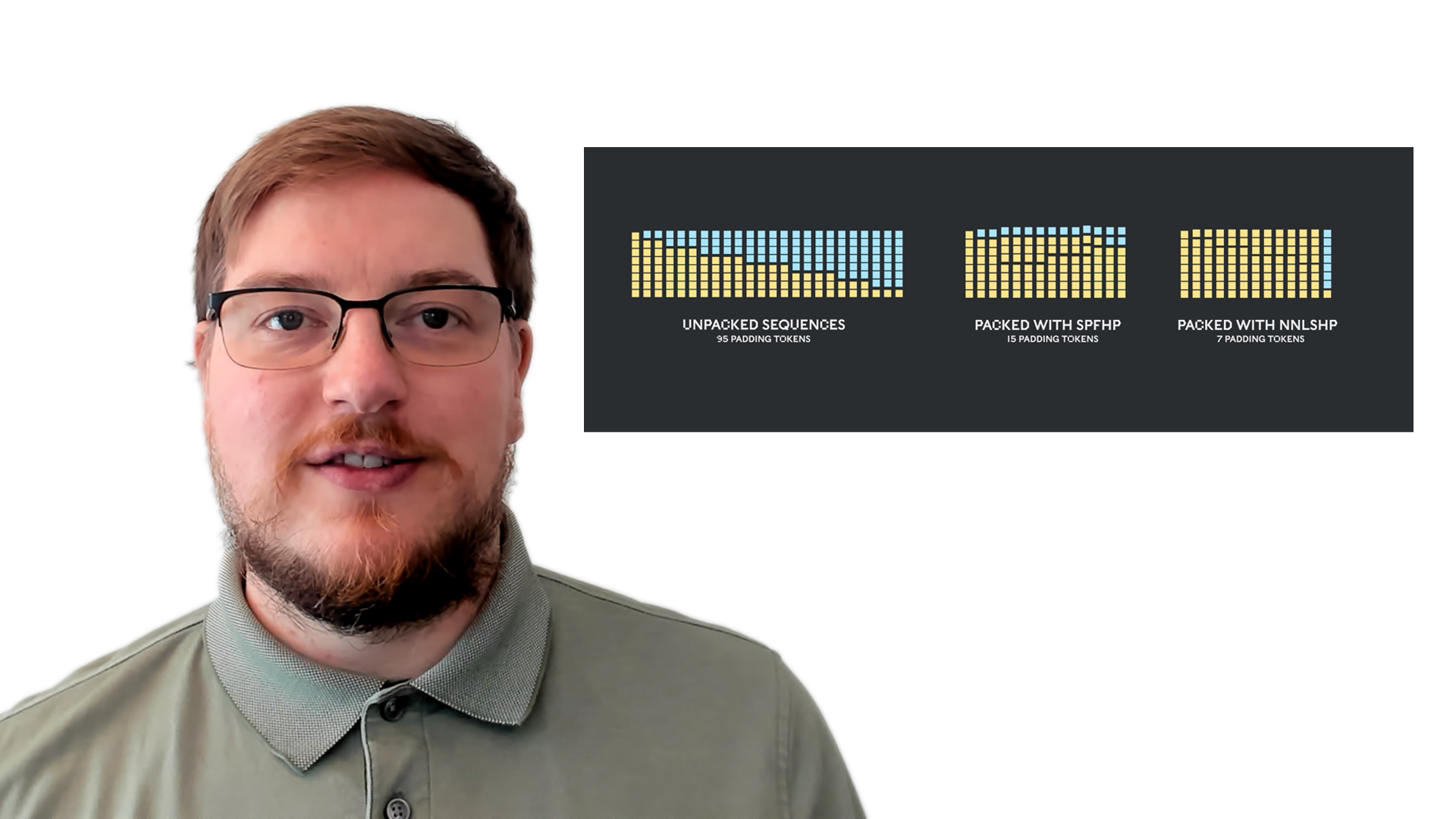
We introduced Graphcore's highly efficient Non-Negative Least Squares Histogram-Packing algorithm (or NNLSHP) as well as our BERT algorithm applied to packed sequences in a new paper.

Computational Waste in NLP due to sequence padding

We began to investigate new ways of optimising BERT training while working on our recent benchmark submissions to MLPerf^TM. The goal was to develop useful optimisations that could easily be adopted in real-world applications. BERT was a natural choice as one of the models to focus on for these optimisations, as it is widely used in industry and by many of our customers.

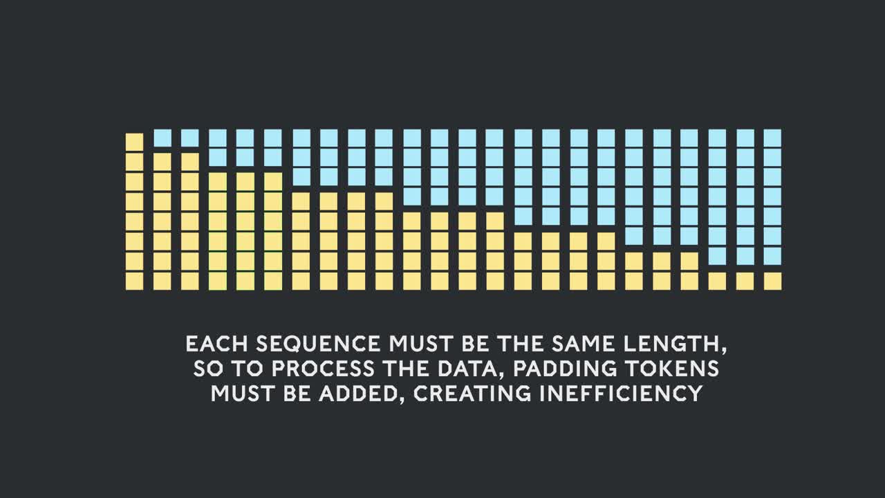
It really surprised us to learn that in our own BERT-Large training application using the Wikipedia dataset, 50% of the tokens in the dataset were padding - resulting in a lot of wasted compute.

Padding sequences to align them all to equal length is a common approach used with GPUs but we thought it would be worth trying a different approach.

Sequences have a large variation of length for two reasons:

1. The underlying Wikipedia data shows a large variation in document length.
2. The BERT-pre-processing itself randomly reduces the size of extracted documents that are combined to generate a training sequence.

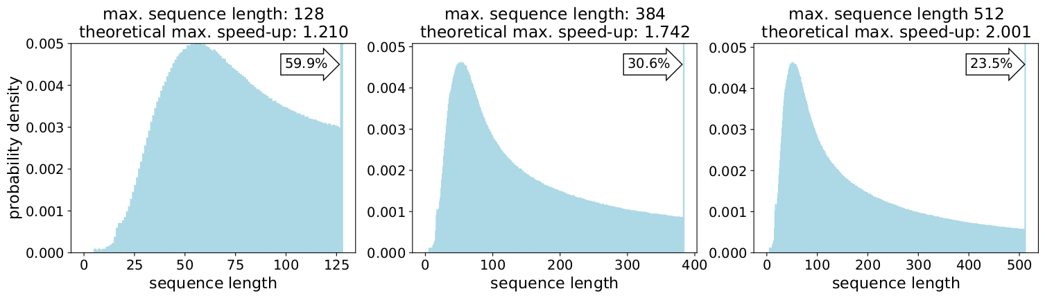
Filling up the length to the maximum length of 512 results in 50% of all tokens being padding tokens. Replacing the 50% of padding by real data could result in 50% more data being processed with the same computational effort and thus 2x speed-up under optimal conditions.

Is this specific to Wikipedia? No.

Well, then is it specific to language? No.

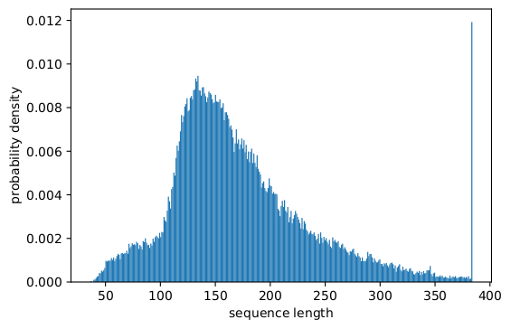
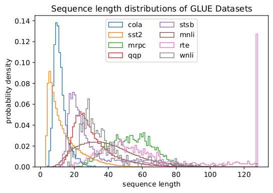
In fact, skewed length distributions are found everywhere: in language, genomics and protein folding. Figures 2 and 3 show distributions for the SQuAD 1.1 dataset and GLUE datasets.

How can we handle the different lengths while avoiding the computational waste?

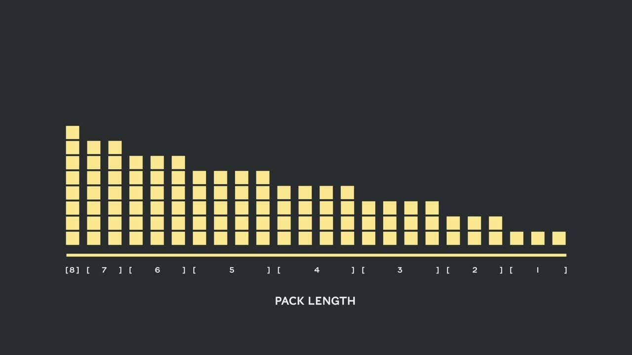
Current approaches require different computational kernels for different lengths or for the engineer to programmatically remove the padding and then add it back in repeatedly for each attention block and loss calculation. Saving compute by blowing up the code and making it more complex was not appealing so we searched for something better. Can't we just put multiple sequences together in a pack with a maximum length and process it all together? It turns out, we can! 

This approach requires three key ingredients:

1. An efficient algorithm to decide which samples to put together to have as little remaining padding as possible
2. Adjusting the BERT model to process packs instead of sequences
3. And adjusting the hyperparameters.

Packing

At first, it seemed unlikely that you would be able to pack a large dataset such as Wikipedia very efficiently. This problem is commonly known as bin-packing. Even when packing is limited to three sequences or less, the resulting problem would be still strongly NP-complete, lacking an efficient algorithmic solution. Existing heuristics packing algorithms were not promising because they had a complexity of at least \(O(n log(n))\), where n is the number of sequences (~16M for Wikipedia). We were interested in approaches that would scale well to millions of sequences. 

Two tricks helped us to reduce the complexity drastically: 

1. Limiting the number of sequences in a pack to three (for our first solution approach).
2. Operating solely on the histogram of sequence length with one bin for each occurring length.

Our maximum sequence length was 512. So, moving to the histogram reduced the dimension and complexity from 16 million sequences to 512 length counts. Allowing a maximum of three sequences in a pack reduced the number of allowed length combinations to 22K. This already included the trick to require the sequences to be sorted by length in the pack. So why not try 4 sequences? This increased the number of combinations from 22K to 940K, which was too much for our first modelling approach. Additionally, depth 3 already achieved remarkably high packing efficiency.

Originally, we thought that using more than three sequences in a pack would increase the computational overhead and impact the convergence behaviour during training. However, to support applications such as inference, which require even faster, real-time packing, we developed the highly efficient Non-Negative Least Squares Histogram-Packing (NNLSHP) algorithm.

Non-Negative Least Squares Histogram-Packing (NNLSHP)

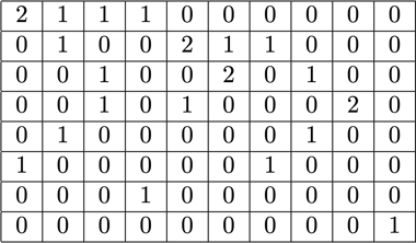
Bin packing is quite often formulated as a mathematical optimization problem. However, with 16 million sequences (or more) this is not practical. The problem variables alone would exceed most machines’ memory. The mathematical program for a histogram-based approach is quite neat. For simplicity, we decided for a least squares approach (\(Ax=b\)) with histogram vector \(b\). We extended it by requesting the strategy vector x to be non-negative and adding weights to allow for minor padding.

The tricky part was the strategy matrix. Each column has a maximum sum of three and encodes which sequences get packed together to exactly match the desired total length; 512 in our case. The rows encode each of the potential combinations to reach a length the total length. The strategy vector \(x\) is what we were looking for, which describes how often we choose whichever of the 20k combinations. Interestingly, only around 600 combinations were selected at the end. To get an exact solution, the strategy counts in x would have to be positive integers, but we realised that an approximate rounded solution with just non-negative \(x\) was sufficient. For an approximate solution, a simple out-of-the-box solver could be used to get a result within 30 seconds.

At the end, we had to fix some samples that did not get assigned a strategy but those were minimal. We also developed a variant solver that enforces that each sequence gets packed, potentially with padding, and has a weighting dependent on the padding. It took much longer, and the solution was not much better.

Shortest-Pack-First Histogram Packing

NNLSHP delivered a sufficient packing approach for us. However, we were wondering if we could theoretically get a faster online capable approach and remove the limitation of putting only 3 sequences together.

Therefore, we took some inspiration from existing packing algorithms but still focused on the histograms.

There are four ingredients for our first algorithm, Shortest-pack-first histogram-packing (SPFHP):

1. Operate on the counts of the histogram from longest sequences to shortest.
2. If the current sequence length does not fit into any pack, start a new set of packs.
3. If there are multiple fits, take the pack where the sum of sequence length is the shortest and modify the counts respectively.
4. Check again for fits of the remaining counts.

This approach was the most straightforward to implement and took only 0.02 seconds.

A variant was to take the largest sum of sequence length instead of the shortest and split counts to get more perfect fits. Overall, this did not change efficiency much but increased code complexity a lot.

Wikipedia, SQuAD 1.1, GLUE packing results 

Table 1, 2 and 3 show the packing results of our two proposed algorithms. Packing depth describes the maximum number of packed sequences. Packing depth 1 is the baseline BERT implementation. The maximum occurring packing depth, wen no limit is set is denoted with an additional “max”. The number of packs describes the length of the new packed dataset. Efficiency is the percentage of real tokens in the packed dataset. The packing factor describes the resulting potential speed-up compared to packing depth 1.

We had four main observations:

1. The more skewed a distribution, the higher the benefits of packing.
2. All datasets benefit from packing. Some even by more than a factor of 2.
3. SPFHP gets more efficient when the packing depth is not limited.
4. For a maximum number of 3 packed sequences, the more complex NNLSHP is, the more efficient it is (99.75 vs. 89.44).

Table 1: Key performance results of proposed packing algorithms (SPFHP and NNLSHP) on Wikipedia

Table 2: Performance results of proposed packing algorithms for SQUaD 1.1 BERT pre-training.

Table 3: Performance results of proposed packing algorithms for the GLUE dataset. Only the baseline and the SPFHP packing results without limiting the packing depth are displayed.

BERT processing adjustment

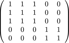
Something interesting about the BERT architecture is that most processing happens on a token level, which means it does not interfere with our packing. There are only four components that need an adjustment: the attention mask, the MLM loss, the NSP loss and the accuracy.

The key for all four approaches to handle different numbers of sequences was vectorization and using a maximum number of sequences that can be concatenated. For attention, we already had a mask to address the padding. Extending this to multiple sequences was straightforward as can be seen in the following TensorFlow pseudo code. The concept is that we made sure that attention is limited to the separate sequences and cannot extend beyond that.

For the loss calculation, in principle we unpack the sequences and calculate the separate losses, eventually obtaining the average of the losses over the sequences (instead of packs).

For the MLM loss, the code looks like:

For the NSP loss and the accuracy, the principle is the same. In our public examples, you can find the respective code with our in-house PopART framework.

Wikipedia overhead and speedup estimate

With our modification of BERT, we had two questions:

1. How much overhead does it bring with it?
2. How much does the overhead depend on the maximum number of sequences that are put together in a pack?

Since data preparation in BERT can be cumbersome, we used a shortcut and compiled the code for multiple different packing depths and compared the respective (measured) cycles. The results are displayed in Table 4. With overhead, we denote the percentage decrease in throughput due to changes to the model to enable packing (such as the masking scheme for attention and the changed loss calculation). The realized speed-up is the combination of the speed-up due to packing (the packing factor) and the decrease in throughput due to the overhead.

Table 4: Estimated speed-up comparison of proposed packing algorithms (SPFHP and NNLSHP) on Wikipedia

Thanks to the vectorization technique, the overhead is surprisingly small and there is no disadvantage from packing many sequences together.

Hyperparameter-adjustments

With packing, we are doubling the effective batch size (on average). This means we need to adjust the training hyperparameters. A simple trick is to cut the gradient accumulation count in half to keep the same effective average batch size as before training. By using a benchmark setting with pretrained checkpoints, we can see that the accuracy curves perfectly match.

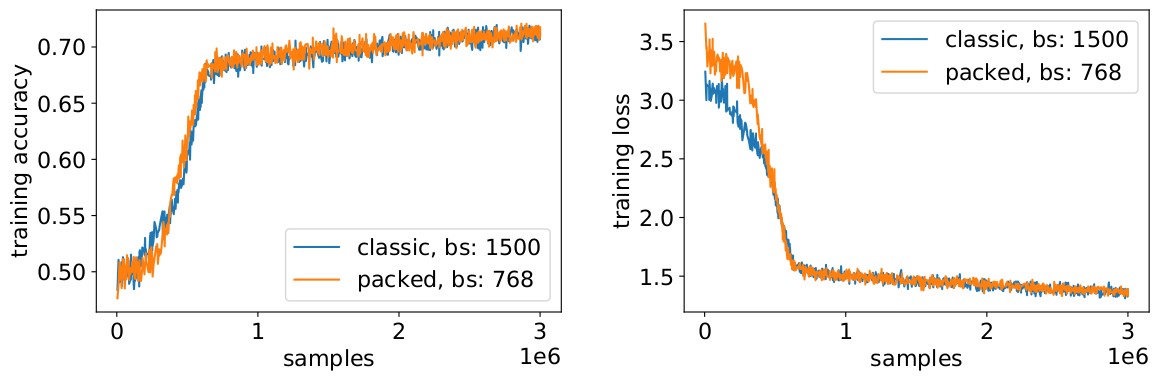
The accuracy matches: the MLM training loss may be slightly different at the beginning but quickly catches up. This initial difference could come from slight adjustments of the attention layers which might have been biased towards short sequences in the previous training.

To avoid a slowdown, it sometimes helps to keep the original batch size the same and adjust the hyperparameters to the increased effective batch size (doubled). The main hyperparameters to consider are the beta parameters and the learning rates. One common approach is to double the batch size, which in our case decreased performance. Looking at the statistics of the LAMB optimizer, we could prove that raising the beta parameter to the power of the packing factor corresponds to training multiple batches consecutively to keep momentum and velocity comparable.

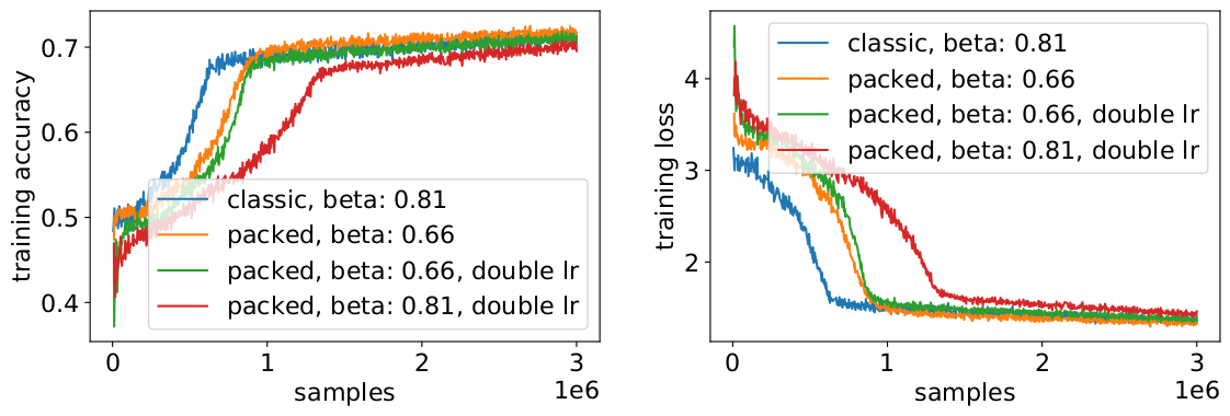
Our experiments showed that taking beta to the power of two is a good heuristic. In this scenario, the curves are not expected to match because increasing the batch size usually decreases convergence speed in the sense of samples/epochs until a target accuracy is reached. 

Now the question is if in the practical scenario, do we really get the anticipated speed-up?

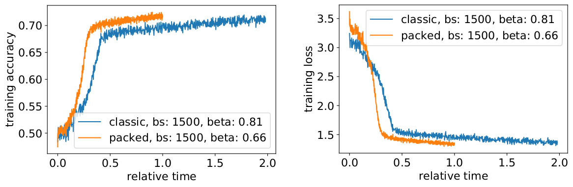
Yes, we do! We gained an additional speedup because we compressed the data transfer.

Conclusion

Packing sentences together can save compute effort and the environment. This technique can be implemented in any framework including PyTorch and TensorFlow. We obtained a clear 2x speed-up and, along the way, we extended the state of the art in packing algorithms.

Other applications that we are curious about are genomics and protein folding where similar data distributions can be observed. Vision transformers could also be an interesting area to apply differently sized packed images. Which applications do you think would work well?

Read the Paper

Access the Code on GitHub

Thank you

Thanks to our colleagues in Graphcore’s Applications Engineering team, Sheng Fu and Mrinal Iyer, for their contributions to this work and thank you to Douglas Orr from Graphcore’s Research team for his valuable feedback.