.png?width=1440&name=Blog%20Header%20170122%20(1).png "Blog Header")
Jan 17, 2022
Jan 17, 2022
We're Hiring
Join us and build the next generation AI stack - including silicon, hardware and software - the worldwide standard for AI compute
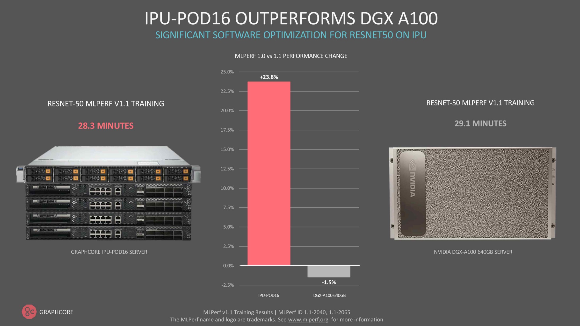
Join our teamGraphcore engineers delivered outstanding performance at scale for the latest MLPerf v1.1 training results published in December 2021 [9], with our IPU-POD16 outperforming Nvidia’s flagship DGX A100 on ResNet-50.
 Here, we will explain how our team achieved these accelerations at scale for this popular computer vision model. In this technical guide, we’ll uncover the various techniques and strategies used by Graphcore engineers covering efficient hardware scaling, memory optimization, experiment tracking, performance optimisation and more.
While focusing on benchmark optimizations for ResNet-50 in MLPerf for the IPU [9], this guide gives a general perspective behind the thought process for benchmark optimisations that can also translate to other applications and hardware.
For our MLPerf v1.1 results, published in December 2021 [9], we achieved a time to train of 28.3 minutes for ResNet-50 training on ImageNet (RN50) with 30k images per second throughput and 38 epochs till convergence at 75.9% validation accuracy on an IPU-POD16.
Before we started on our first MLPerf project in 2020, throughput for ResNet-50 training was around 16k images per second and it took approximately 65 epochs to reach convergence. Putting these numbers together gives us a 3.2x overall improvement. We then scaled the application from an IPU-POD16 to our IPU-POD256, which gave us another 7.5x improvement in time to train and 12x improvement in throughput. So how did we achieve this speed-up?
The tools that we developed along the way are provided in our public examples and are not that specific to RN50 or the MLPerf benchmark. We thought other IPU developers out there might find them useful for their models. The key ingredients are:
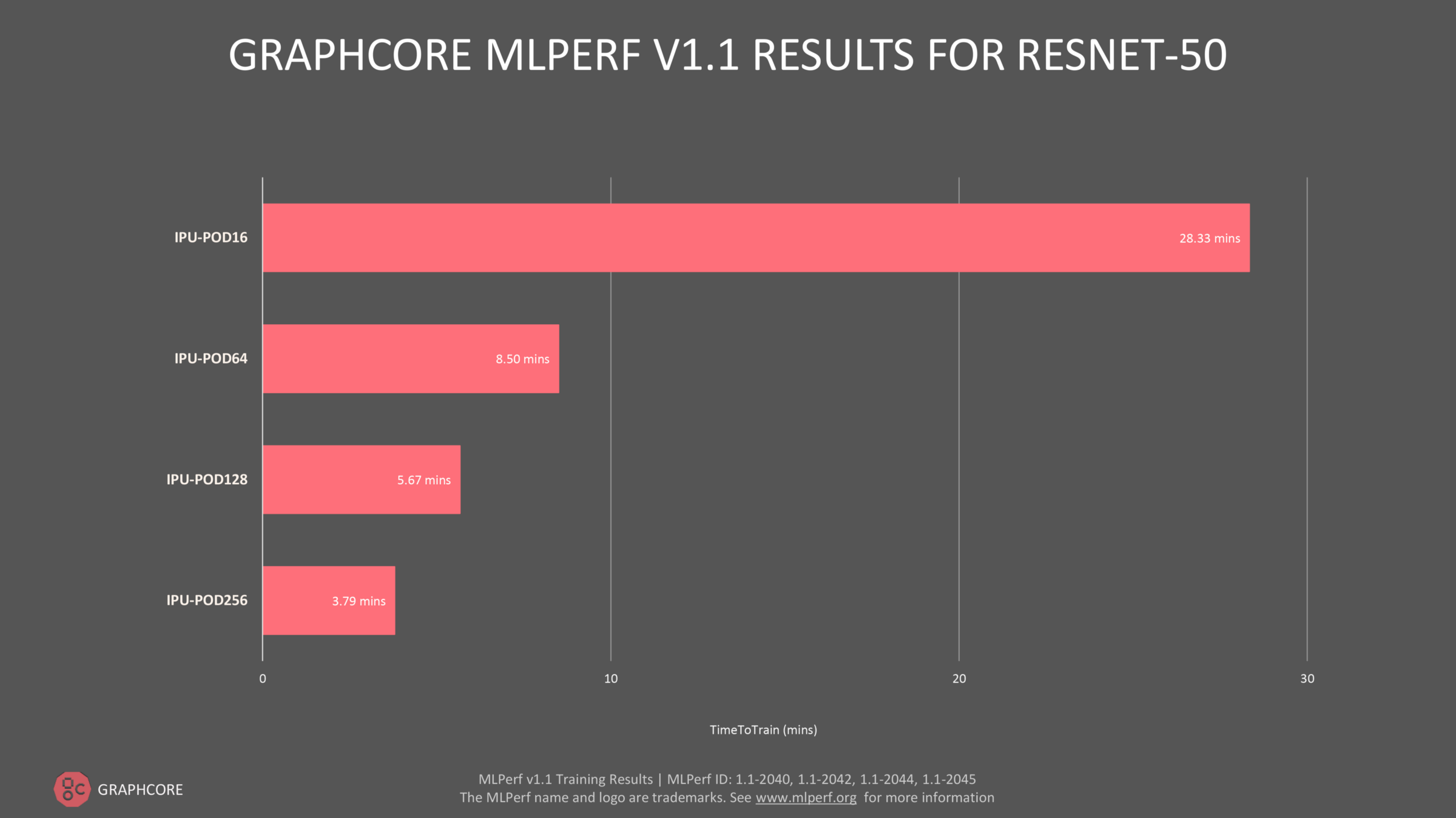
Image: Scaling the application from an IPU-POD16 to our IPU-POD256
To scale our application, numerous features had to be put in place. A major challenge when scaling is the increased batch size and communication which requires time for data transfer and memory for the code. For the local replicas, we want to keep the micro batch size as large as possible to obtain good statistical estimates for the batch norm which is a key part of the ResNet-50 model. The gradients for each replica need to be aggregated and the optimizer performs its update.
This comes with computational and communication overhead. One trick to reduce this is gradient accumulation on the single replicas and have a bigger effective batch size. By adding more replicas, the effective batch size would scale linearly. Whereas this approach would guarantee almost linear scaling, the higher effective batch size increases the number of epochs required to get convergence. Hence, gradient accumulation needs to be reduced for larger systems and effective communication of the gradients is essential.
In our experiments, the best compromise for IPU-POD128 and IPU-POD256 was to have a gradient accumulation count of 2, to have a slightly reduced communication but to keep the effective batch size as small as possible. Given the larger batch size, the changes mentioned in “LARS Optimizer and Hyperparameter Optimization” were necessary since SGD would increase the required epochs much more than LARS. Also, we made extensive use of our load distribution tool PopDist as described in “Scaling Host-IPU Communication”. By increasing the number of hosts with local data storage, we improve the data loading bandwidth and make sure that there is no slowdown in data transfer, no matter how many accelerators are used.
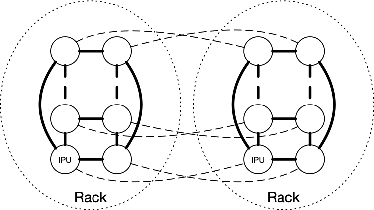
Graphcore’s IPU-PODs have been designed from the ground up with that scalability in mind, as shown by the incredible scaling exhibited in our latest MLPerf submission. Within a rack, IPUs are directly connected to each other to form two rings via high-bandwidth IPU-Link connectivity. Using these direct connections, each IPU-POD64 provides a huge IPU-Link bandwidth of 10.24TB/s, with ultra-low latency (250ns). On top of these vertical intra-rack connections, IPUs are connected across racks (directly or through a switch) to form a horizontal ring. This means that doubling the number of racks more than doubles the amount of bandwidth available.
Graphcore Communication Library (GCL) has been designed to make full use of these hardware features.
IPU-POD128 and IPU-POD256 are built from multiple IPU-POD64s. A single IPU-POD64 consists of 16 IPU-M2000 stacked vertically and connected with IPU-Links to form a 2D-Torus. The flexibility of our scale-out solution allows us to connect IPU-POD64s together horizontally to form larger systems. There are two possible methods to connect such systems: directly (GW-Links on one IPU-M connect directly to IPU-M2000s on other IPU-POD64 systems) or over a switched fabric where GW-Links on all IPU-M2000s connect to switches that then forward the traffic to correct destination IPU-M2000s on other IPU-POD64s. In both cases, the syncs between multiple IPU-POD64s are sent over the GW-Links without requiring physical sync lines to enable a simpler scale-out. For the IPU-POD128 and IPU-POD256 we use for MLPerf work, we use the switched solution as it allows us to be more flexible and provides better fail-over.
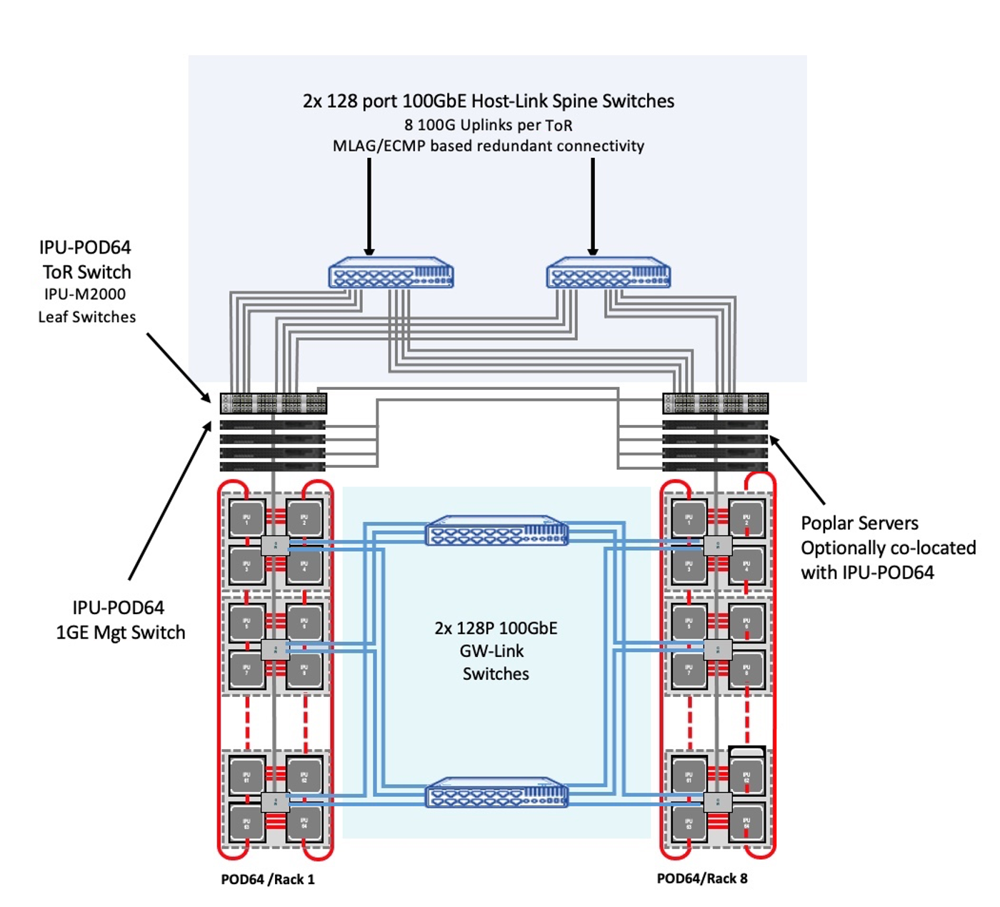
Image: Graphcore’s scale-out solution for IPU-POD128 to IPU-POD512
Looking at the individual aspects of IPU-POD scale-out topology, now we can take a snapshot of what this looks like in practice. This illustrates that even with all the flexibility and great options deploying over an existing switched fabric brings, it is actually not as intensive as might at first be thought in terms of ‘extra kit’ needed. This system has 8x IPU-POD64 racks so we can call it an IPU-POD512. Interconnecting all of the GW-Links between each IPU-M2000 in an IPU-POD512 can be achieved using just two 128 port- 100GbE switches.
To speed up training of AI models, one idea is to replicate the model on many IPUs, each processing a different batch. After having processed a batch, replicas share what they have learned from the batch (the gradients) using an all reduce. In the ideal case, if the All-Reduce was instantaneous, we would have perfect scaling in the sense of throughput: doubling the number of replicas would allow us to process double the amount of training samples.
Several optimizations enabling the scale-out beyond a single IPU-POD64 have been implemented in GCL. All model replica internal data exchange is known and detailed by Poplar at compile time and with the assumption that all collective communication, ML model details, and network topology also are known at compile time, the GCL execution is deterministic and can be scheduled and optimized accordingly. GCL also exposes a public API for specifying communication groups as sub-sets of the total set of replicas giving us the flexibility to perform operations on large systems. For the larger scaling to IPU-POD256, we use a phased all reduce where the tensor reduction over a multi-POD system is performed as three distinct operations.
First, a ReduceScatter is done over the IPU-Links within each of the IPU-POD64s that are the building blocks of an IPU-POD256. The output of the Reduce Scatter becomes an input to the All-Reduce that is run over the GW-Links. This exchanges the data elements between multiple PODs making sure every replica at the same level contains the same data. Finally, an All-Gather collective operation is performed on the output of the All-Reduce and again it runs within each individual IPU-POD64 so that every replica in the end contains the same copy of the data.
A crucial characteristic of our implementation is that the time spent in the All-Reduce is a function of the total amount of data to share divided by the total bandwidth available. Because doubling the number of IPUs means double the amount of bandwidth, the time for the All-Reduce remains constant. Having that constant time All-Reduce is the key feature of Graphcore’s offering: it enables innovators to experiment faster by using more hardware effectively reducing the feedback loop ultimately leading to exciting discoveries.
Given our small gradient accumulation count of 2 for large systems, any optimization of the communication of the gradients had a major impact on our scaling performance. For example, we grouped tensors of different types and shapes together and did the communication in one shot. Also, to make full use of the bandwidth, we optimized the gateway between host and IPU, to immediately forward the data and thus significantly reducing the latency across a variety of applications. Each IPU-POD64 comes with its own gateway. So, this change is mostly benefiting the scaling from IPU-POD16 to IPU-POD64.
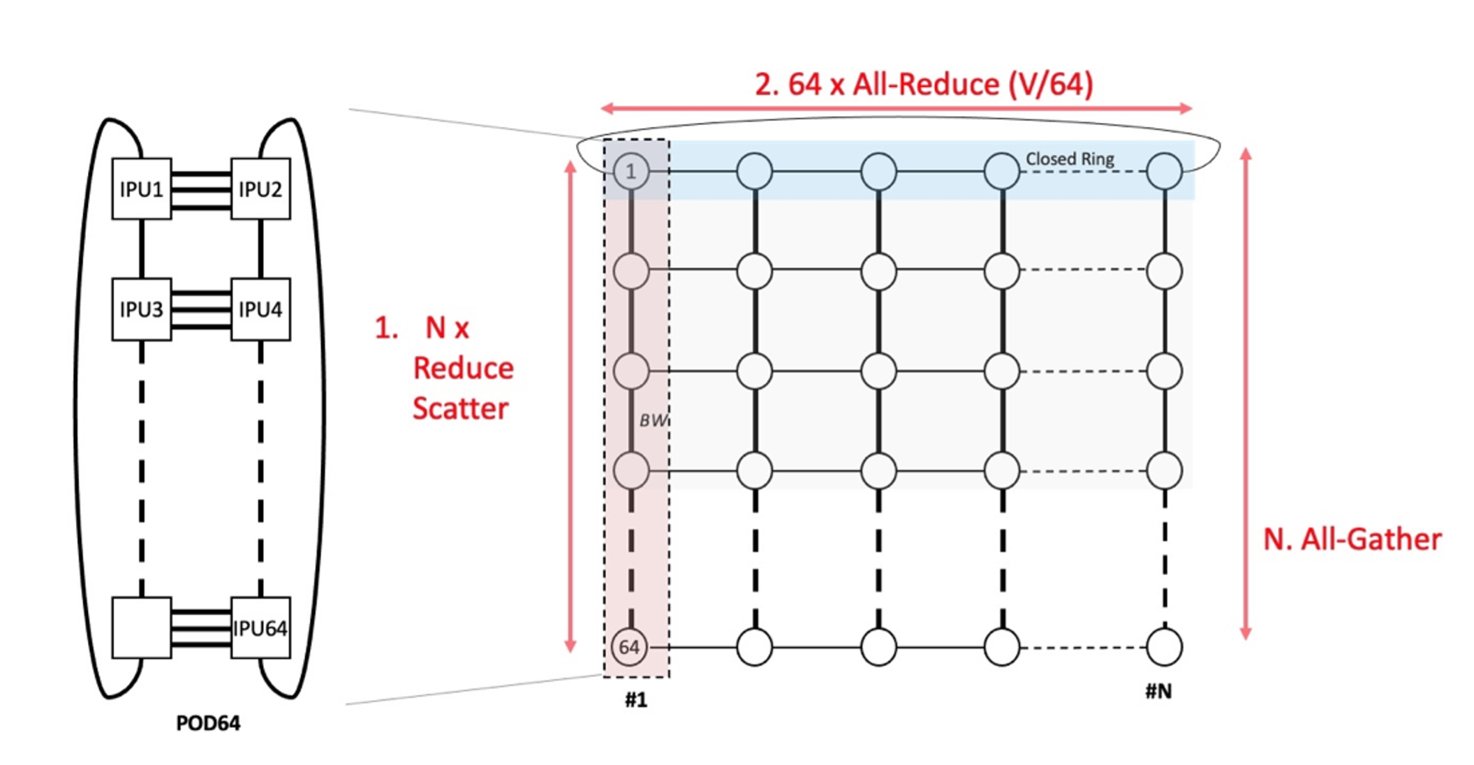
Image: Visual representation of the Three-Phase All-Reduce.
Whereas the memory required by the data stays the same when scaling, additional memory is required for the exchange code. Thus, memory optimizations as for example mentioned in “Other Memory and Speed Optimizations” were crucial for our scaling success, especially since the LARS optimizer required even more memory than SGD. A specific optimization for scaling to IPU-POD128 and IPU-POD256 was the reduction of the code size for the exchange between IPU-PODs.
For validation, no backward pass is needed and in the batch norm layers, the synchronized moving mean and variance are applied. Thus, the computational layout is substantially different. To not waste time with graph swapping, we instead apply an offline evaluation scheme, i.e., we store the checkpoints during training and afterwards, we evaluate the performance using the validation data. We also keep the same configuration of the IPUs to avoid time for reconfiguration. That means for the case of the POD₂₅₆, we have 128 host processes where each one is responsible for one validation file and results then get aggregated to calculate the overall performance. Since we are working with static graphs, the 50000 validation images cannot be perfectly split even with a batch size of 1, which would be inefficient. However, for the MLPerf setting, all images need to be processed and samples cannot be omitted. Thus, we pad our data to the next larger batch and then remove the padding results in the post-processing.
During the whole project, it was important to keep track of experiments, look up the detailed parameter configurations and dive deep into the logs. Thus, we took great advantage of the experiment tracking with Weights and Biases and regularly created reports to communicate results to colleagues and compare runs to figure out any potential difference. What made the experiments challenging was that with a low epoch count, convergence gets overly sensitive to any changes. For example, cutting the accumulation count in half could easily transition a non-converging setup to a converging one. Also, there was a large variation in between experiments which required this approach to experiment tracking. We tracked more than 2600 experiments. Recently, we extended our tracking in our CNN repository. With the --wandb and --wandb-project option, results get uploaded right away instead of waiting for the final result to be uploaded.
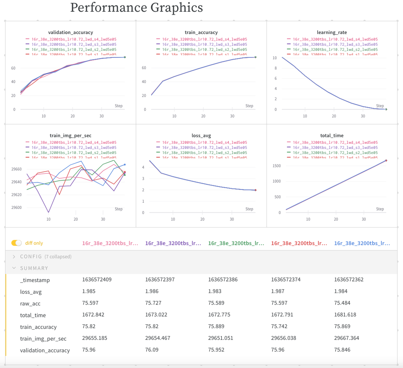
Image: Weights and Biases Report
In practice, people usually train their network around 90 epochs or even more. Since the MLPerf benchmark only cares about the time to train, there is a lot of tweaking happening to reduce this number. Our goal was to reduce the number to 44 epochs or even fewer given previous results in the competition. Our original implementation used group norm instead of batch-norm for faster processing and avoiding dependence between samples. For a discussion, see [1].
For 65 epochs or more, this normalization works perfectly. However, while fine-tuning hyperparameters, we learned that a more aggressive and costly normalization is required to get convergence in the desired small epoch count. That means the tools that we developed to enable large batch-norm were specific to the MLPerf benchmark in the sense of having to reduce the number of epochs. Without this requirement, we could have stuck to group norm.
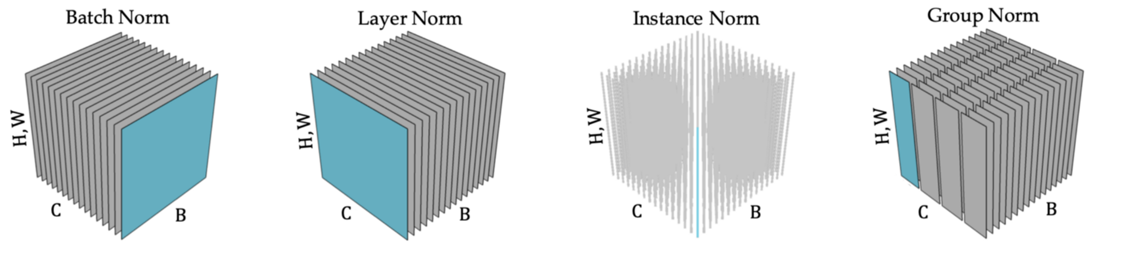
mage: Each subplot corresponds to a specific technique of normalisation characterised by its groups of components sharing the same normalisation statistics. In each subplot, the tensor of intermediate activations is constituted of the batch axis B, the channel axis C, and the spatial axes (H, W). Image by author, adapted from [7].
Our original setup was a pipeline over 4 IPUs (Intelligence Processing Units) with a replication factor of 4 for data parallel processing and grouped schedule. We used a batch size of 16. Changing that setting to batch-norm was a simple configuration change but still convergence improved only slightly. It got better when we fine-tuned the memory and pipeline stages to get a batch size of 24 by using memory efficient communication, limiting the code memory size for each IPU, and adjusting the length of pipeline stages. Still, we could not reach the anticipated 44 epochs. So, we ran some simulations and discovered that a batch size of 32 should be sufficient. With the simulation, we could reach convergence in 44 epochs, but the throughput was below acceptable, and we needed some tweaks as described in the “Increasing the Throughput” section.
For getting good hardware acceleration, it is common to work with large batches of data. Using more data on a single accelerator usually increases the usage of the ALU (Arithmetic Logic Unit) and makes sure that the accelerator gets enough workload. Note that the IPU has a unique way of distributing workloads and can also accelerate workloads with small batch sizes. Additionally, communication of gradients and optimizer updates can be expensive and thus throughput can be increased by making these updates less frequent, for example by using gradient accumulation. Note that gradient accumulation gives diminishing returns with every increase though. In our experiments, we realized that larger batch-sizes require more epochs for the training as can be also seen in the MLPerf Reference Convergence Points [8]. Thus, the benefit of larger batches can outweigh the gain of speed. On the other hand, a minimum batch size of 32 is required per “replica” to make batch norm work.
For the optimal IPU-POD16 config, we ended up with an effective batch size of 3200 (16 replicas, each with a micro-batch size of 20, and a gradient accumulation count of 10) which converged in 38 epochs. For scaling to larger systems, we reduced the gradient accumulation count, respectively. Due to communication efficiency and optimizations on the larger machines, it was sufficient to keep a gradient accumulation count of 2. For the IPU-POD64 system, we used a similar effective batch size of 3840 (64 replicas, gradient accumulation count of 3) to also converge in 38 epochs. For IPU-POD128 and IPU-POD256, we used a gradient accumulation count of 2 with an effective batch size of 5120 and 10240 and respective epochs till convergence of 41 and 45. Using larger sizes would have increased the epoch counts much more and was not feasible.
Whereas normal ML settings show some robustness in the choice of hyperparameters, the low epoch count in MLPerf makes the convergence sensitive to any changes. This can be best seen by the choice of optimizer. LARS is known to be a good optimizer for large batch sizes. During our project, we learned that it is also a better optimizer than Stochastic gradient descent with Momentum (SGD) in the sense of requiring fewer epochs till convergence. This benefit grows with increasing batch size. Note that LARS requires more memory and compute, but the minor costs exceed the major savings. One major change between our first and second MLPerf submission was to optimize memory usage and enable LARS which resulted in a great speed-up. For example, for our POD₁₆ setup, LARS reduced the number of required epochs from 44 to 38. One key ingredient is the number of warmup epochs. Whereas SGD requires 5 epochs, LARS can work with only 2 epochs. Another sensitive hyperparameter is the weight decay parameter in LARS, reducing it by a factor of two and adjusting the learning rate, accelerates convergence by up to 2 epochs.
In contrast to the natural language processing model, BERT, optimizing pipelines for RN50 can be challenging. There are a lot of different components that require different code and the size of the data in between the layers changes a lot. So, modifying the split strategy just a little bit could have a major impact on the memory profile, jumping from a lot of memory left to requiring too much memory. Also, processing load can be highly imbalanced as we discovered with the PopVision Graph Analyser. The fourth IPU took twice as long for the processing compared to the second and there was no room for balancing due to memory requirements of the data. On the other hand, IPU0 could not do too much processing because it had the largest stash of activations to store. Similarly, IPU1 and IPU2 also had some idle time which is even larger than the synchronization depicted by the green bar. Due to the imbalanced computation and memory requirements, it is hard to improve further, and we chose a different route, using a recomputation approach that can work on a single IPU and uses distributed batch norm to enable a sufficiently large batch size.
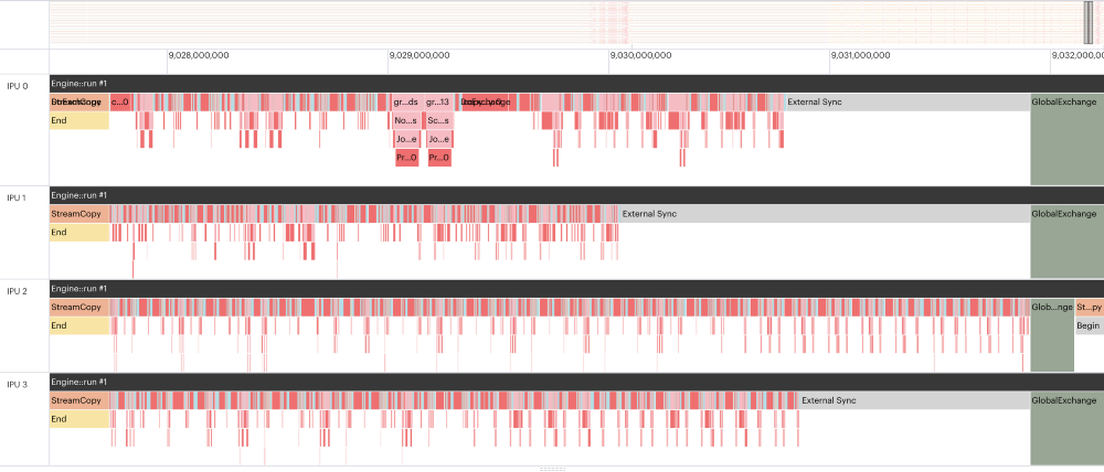
Image: PopVision Graph Analyser excerpt of a grouped schedule pipeline over 4 IPUs with batch size 20. The third row (IPU 2) corresponds to the last, 4th stage. IPU 1 needs less than 60% of the processing cycles compared to IPU 2. Image by author.
Our batch norm implementation is fused and optimized on the Poplar level. With all the memory fine-tuning we used before for the pipeline setup, we realized that we could now increase the batch size on a new setup on a single IPU from 6 to 12 without any pipelining. Now, to get to a batch size of 32 for the batch norm, we only required a distributed batch norm. For everything else, normal data parallel processing would be sufficient. We added this feature into our framework with just a few lines of code where we aggregated the statistics across multiple replicas within the normalization implementation. This approach was very efficient and did not require much more memory, especially since the vectors for the statistics are quite small. Also, the backwards pass was just an aggregation of gradients between the IPUs that contributed to the distributed batch norm and thus resulted only in a single line of code.
For the application code in TensorFlow 1.15, the interface was kept minimalistic. Only a configuration number must be set:
For a batch size of 12, we would need to aggregate data between at least 3 IPUs to reach a batch norm batch size of at least 32. To avoid communication between IPU-M2000 machines, it would have to be 4 IPUs instead.
For better throughput and less communication overhead from the distributed batch norm, we wanted to increase the batch size and limit the distributed batch norm to two IPUs. Thus, we took advantage of recomputation. Since there is no native support for this in TensorFlow 1.15, we used a programming trick. The IPU implementation of pipelining comes with a sequential schedule which can be used to shard a computational graph over multiple IPUs. Instead, we did not distribute the processing over multiple IPUs but kept them all on one IPU. Note that the code size in the on-chip memory barely increases but a lot of intermediate activations do not get stored but recomputed. Thus, we are freeing a lot of memory that can be used to increase the batch size. By setting our splits to b1/0/relu, b1/2/relu, b2/0/relu, b2/2/relu, b3/0/relu, and b3/3/relu, we increased the batch size to 20. We could have used fewer recomputation points by offloading some of the optimizer state to the host. We refrained from that possibility and kept everything in memory because we made better use of the communication bandwidth by bringing more data to the IPU. So, all that is required for recomputation are three ingredients:
“PipelineSchedule.Sequential” as the “pipeline_schedule”device_mapping = [0] * len(computational_stages)— in our case, there were 7 computational stagesBalancing recomputation points requires the knowledge of memory occupation of the different stages in the computational graph. For fine-tuning, we used the memory profiles in the PopVision Graph Analyzer to make sure we make optimal use of the memory. As a result, we have more dense set of recomputation checkpoints at the initial layers and keep a longer final stage to reduce the amount of computational overhead because for the last stage the forward pass never gets recomputed.
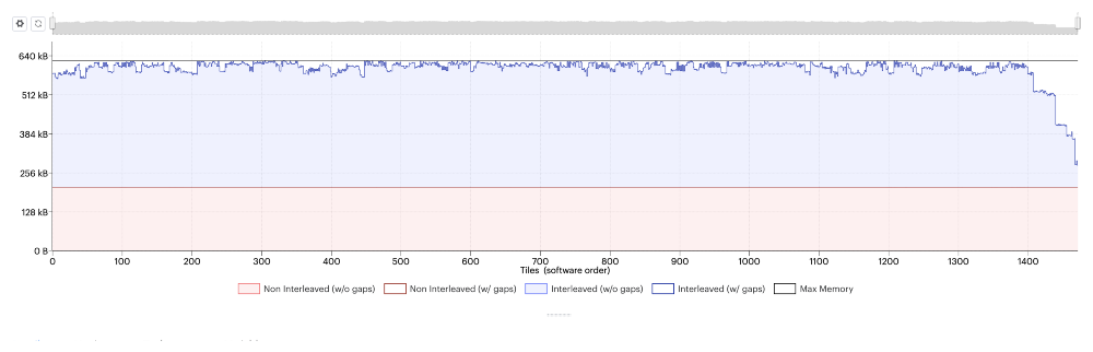
Image: The memory utilization for 1472 tiles of a single IPU. It’s reaching the memory limit for each tile. (Generated using the PopVision Graph Analyser).
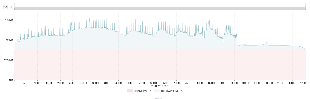
Image: Liveness report created with the PopVision Graph Analyser. We can see the forward pass excluding the last section, followed by 7 bumps for each section of recomputation of forward pass (memory increase) and backward pass (memory decrease).
For the ResNet-50 benchmark data loading on preprocessing a crucial part of the workload. In one of our experiments, we tried an Intel based host with fewer CPU cores which slowed down our processing significantly compared to using an AMD host. Thus, our disaggregated host architecture is especially important to be able to choose the right host for the application at hand.
A simple approach to get more data transferred is to reduce its size. The augmented image data was transferred in Int8 format, and then normalization happened on the IPU instead of the host. The normalization was implemented as a fused operation that cast the data to Float16 and added a fourth channel with zeroes to reduce memory footprint of the subsequent convolutional layer.
Additionally, to transfer more data, the data loading needs to be parallelized using Graphcore’s PopRun framework [6]. Our analysis showed that for each set of two replicas, one host process is best. Each host was running optimally with 8 numa-aware nodes, 4 for each CPU. Thus, for IPU-POD 16, 64, 128, and 256, we used 1, 4, 8, and 16 hosts, respectively. The command looks something like:
poprun --host $HOSTS $MPI_SETTINGS --num-instances “$INSTANCES” --num-replicas “$REPLICAS” python train.py args
Numa awareness is activated, using “--numa-aware 1” >in the $MPI_SETTINGS. Whereas the host processes are independent MPI processes, a combined representation of the computational graph over all replicas is created across multiple racks. Each host process reads a separate equally sized set of input files. Thus, any conflict in file reading is avoided. The distributed read data is kept in cache even though the effect on performance is negligible.
Apart from recomputation, we used a few more optimization strategies:
with tf.Graph().as_default(), tf.Session():
identical_seed = hvd.broadcast(
identical_seed, root_rank=0, name=”broadcast_seed”).eval()export POPLAR_ENGINE_OPTIONS=’{“target.deterministicWorkers”:”portable”}’“availableMemoryProportion” of the IPUConfig [5] which resulted in a value around 0.15.config.convolutions.poplar_options[‘availableMemoryProportion’] = …For more ideas on memory and processing optimizations, please check out our new guide [4].
All features introduced in this blog are readily available with the latest release. However, we would like to point out that whereas all these technical tricks might help in your application they do not have to. The MLPerf benchmark comes with special rules and limitations that will not hold for practical applications.
In practice, no one would train ResNet-50 on ImageNet to 75.9% validation accuracy. It is easier to download a pretrained network with higher accuracy.
In practice one would train on a different dataset to a higher accuracy. However, when training on a different dataset, the chosen parameters for this benchmark might not transfer. Also, a larger epoch count, and a different learning rate schedule might be desired. With an increase in the number of epochs though, it might be better to go with group norm (or proxy norm) if the training happens from scratch and not with a pretrained model.
A Top1 accuracy of 75.9% is not sufficient for some applications like search. Imagine, you have a search engine on 100.000.000 images like the YFCC100M dataset and you try to search for a certain class of images like for example origami using ResNet-50 with this accuracy. Missing 24% of all relevant images might be ok for you. The challenge will be that because the other class(es) also get misclassified, you will get many more images that are not origami but misclassifications from the other images. In fact, these misclassifications will be the majority [2]. To achieve higher accuracies, it is worth considering more state-of-the-art models like EfficientNet, which benefit from some of the features mentioned in this blog. You might also want to read, “How we made EfficientNet more efficient”[3].
Combining the powerful TensorFlow 1.15 framework with Weights and Biases, Poplar, and the PopVision tools together with the powerful MK2 IPU, we managed to take full advantage of the processing speed and memory and achieved a stunning performance.
A big thanks goes out to Brian Nguyen, Godfrey da Costa (and his team), and Mrinal Iyer who went above and beyond to make this work happen.
We would also like to thank Alex Cunha, Phil Brown, Stuart Cornell, Dominic Masters, Adam Sanders, Håkon Sandsmark, George Pawelczak, Simon Long,
[1] A. Labatie, Removing Batch Dependence in CNNs by Proxy-Normalising Activations, Towards Data Science 2021
[2] D. Ma, G. Friedland, M. M. Krell, OrigamiSet1.0: Two New Datasets for Origami Classification and Difficulty Estimation, arxiv 2021
[3] D. Masters, How we made EfficientNet more efficient, Towards Data Science 2021
[4] Memory and Performance Optimisation Guide, Graphcore
[5] Optimising Temporary Memory Usage for Convolutions and Matmuls on the IPU, Graphcore
[6] PopDist and PopRun: User Guide, Graphcore
[7] N. Dimitriou and O. Arandjelovic, A New Look at Ghost Normalization, arXiv 2020
[8] MLPerf Reference Convergence Points, MLCommons
[9] MLPerf v1.1 Training Results. MLPerf ID: 1.1–2040, 1.1–2042, 1.1–2044, 1.1–2045, 1.1–2065. The MLPerf name and logo are trademarks. See www.mlperf.org for more information.
This blog first appeared in Towards Data Science.
Share: