Using the IPU to accelerate Spatial Interpolation Algorithm of Weather Data

Modernisation and advancements in weather services have led to the wide adoption of grid-point weather data with high spatial and temporal resolution High-precision and grid-based meteorological data are not only the foundation of modern weather forecasting and climate research, but has also opened a variety of potential applications in precision manufacturing, agriculture, and ecological research. For spatial precision, the grid point resolution needs to be increased from the current 0.0083x0.0083 degrees of longitude and latitude (which accounts to 1 square kilometer of land area) to 0.001x0.001 degrees of longitude and latitude. Together with the above spatial precision improvement, improving the temporal precision from a single-day to 14-day forecast  will require 1000 times increase of computing power. In this case, only high-performance computing chips can make fast and timely forecasts. 

We will discuss in this blog the implementation of the Kriging algorithm on Graphcore IPU. The main limitation of the original algorithm is that it can only use single-core computing.

We will show how the total computing time on a single M2000 is 60-time faster than the original algorithm running on an Intel Xeon E5-2680v3 clocked at 2.5GHZ frequency. The source code of the project can be found in Graphcore’s Portfolio Examples Repository.

Introduction to Reference Evapotranspiration (ET₀)

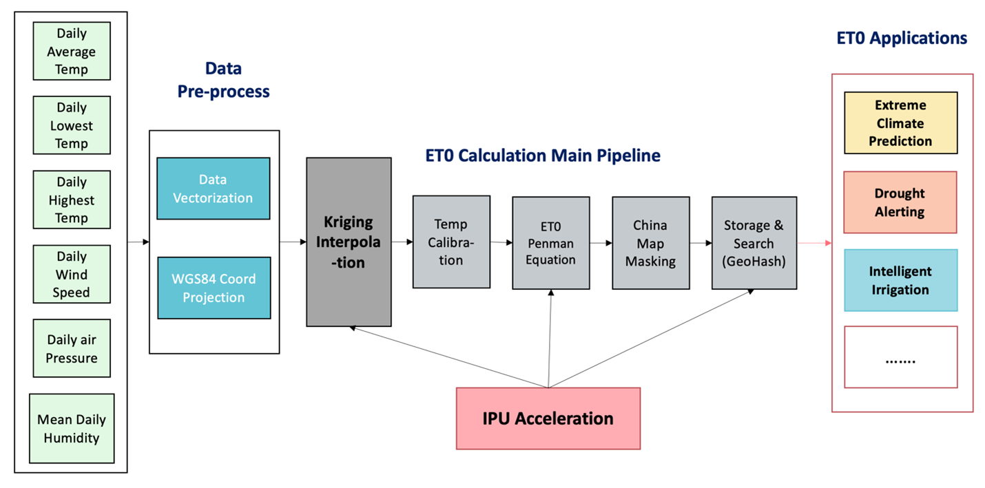
The complete calculation and application process of  the Reference evapotranspiration, or more commonly referred to as ET₀, is shown in its overall flow in Figure 1. Through interpolation analysis and prediction calculation of weather elements namely temperature, humidity, air pressure and wind speed, higher-density meteorological element points are obtained. Using the resulting data points combined with the calibrated temperature, the ET₀ of all grid points in the area are calculated using the Penman Equation. Finally, the ET₀ value in the required area is extracted and stored in the database to be used for the evaluation of meteorological data mining, numerical weather forecasting, and climate change related research. 

ET₀ is also widely applied in areas like extreme weather forecasting, drought forecasting, and smart irrigation. In smart irrigation, ET₀ has significant impact on crop water requirement and water resource management. Accurate ET₀ estimation helps make the correct determination of water resource budget and allocation and hence improves the water utilisation efficiency of irrigation systems. Meteorological data is observed and collected by national weather stations using satellites and radars, and the main challenge is that distribution coverage of these weather stations are limited. Data in areas with higher coverage density has a greater degree of precision while data from low-density regions exhibited lower levels. However, to have a successful and useful application, we need to convert data of monitoring stations into grid-point spatial data with high temporal resolution by using appropriate interpolation methods.

Kriging Algorithm

Kriging algorithm is a regression algorithm for spatial modelling and prediction (interpolation) of random processes or random fields based on covariance function. In specific random processes such as inherently stationary ones, Kriging algorithm can provide optimal linear unbiased estimates. In geostatistics it is referred to as a spatial optimal unbiased estimator and widely applied in areas like geographic, environmental, and atmospheric sciences. The finer the spatial grid points are, the more precise the interpolation prediction results will be. The high precision and the resulting amount of calculations to run the interpolation algorithm means that without enhanced computing power, this algorithm will be limited in a real-world application.

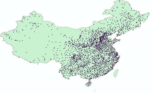
Kriging algorithm is one of the most widely used weather element interpolation predictive algorithms in the industry as well as the built-in interpolation algorithm of ArcGIS, the geographic information analysis software. Figure 2 shows the weather elements at known points, Kriging algorithm uses these points to forecast weather conditions at the rest of the grid points in this map.

Here, we discuss the two-dimensional ordinary Kriging interpolation algorithm adapted from a linear model implementation in the Python open-source code, PyKrige.

Overall Algorithm Flow

The overall calculation formula of Kriging algorithm is shown below (equation 1): 

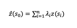
Among them, z(\(S\)_i) is the measured value of the i-th position. In this example, it is the temperature at the given latitude and longitude (as well as humidity, wind speed, etc., a total of 2167 points), and n is the number of measured points in the vicinity of point \(S\)₀. After expanding it into a matrix, it is like the below (equation 2):

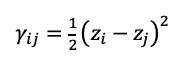
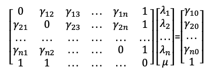Where \(Y\)_ij is the semivariance of z at point (i, j), and its calculation method is shown here (equation 3):

Semivariable Function

It can be seen from the equation (1) that in order to calculate the z value of the known prediction point we need to know the λ vector and the γ matrix. For the known meteorological data, since the z value is available, the γ matrix can be directly calculated by formula (2). For the meteorological data that needs to be predicted, only the longitude and latitude coordinates of the prediction point are known, so the γ matrix of the unknown point needs to be obtained through the coordinates.

To be specific, the linear semivariable function considers that the distance between each point and the semivariance of the corresponding z value of these points have a linear relationship, namely as in equation 4:

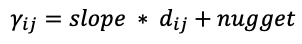
Therefore, the Euclidean distance matrix \(d\)_ij between the known points can be calculated in advance, and then the semivariance matrix of these points can be fitted by the least square method to obtain the values of "slope" and "nugget". For the points that need to be predicted, the distance matrix is calculated and then the semivariance matrix of the prediction point can be calculated through formula (4).

λ vector solution

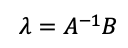
Through step 2, we can get the semivariance matrix A of the known points and the semivariance matrix B of the unknown points, and used in the equation (2) to calculate the λ vector. See equation 5:

Algorithm Flow

The main part of the algorithm is shown in Figure 3. Input data x, y, and z represent longitude, latitude, and weather elements respectively. We use affine transformation to correct the longitude and latitude once, calculate the distance between each corrected point and the semivariance matrix of the corresponding weather elements, and use the least square method to obtain the mapping relationship between the distance and the semivariance matrix. We then use the KD Tree to find the n input points closest to the predicted point (here n is consistent with n in equation (1), where n is set to 12). We calculate respectively the distance matrix between prediction points as well as the distance matrix between prediction points and the above n inputs and then use the mapping parameters to convert them into the semivariance matrix a and b of weather elements (corresponding to A and B in equation (5)). We then calculate λ through the inverse operation and put it in equation (1) to get the final resulting interpolation prediction.

Analysis of Calculation Time Consumption

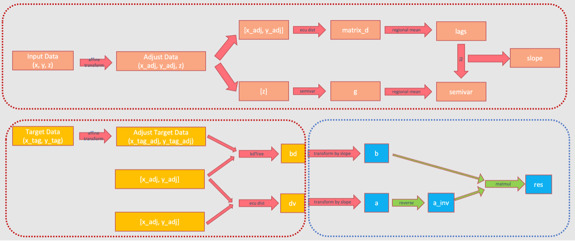
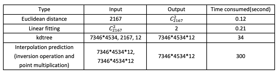
Through the above analysis, it can be seen that the algorithm mainly includes calculation of distance between matrices, least square fitting calculation, KD Tree clustering calculation, and matrix point multiplication and inversion operations. When the input consists of 2167 data points, the resulting predicted data is 7346*4534, each point is predicted by the nearest 12 points nearby, with the calculation scale of each part and the time CPU run time shown in Table 1. It can be seen that the time on CPU is mainly consumed by the KD Tree and interpolation prediction process, while the Euclidean distance and the fitting process consume almost no time. In order to improve the calculation times, we make relevant optimisations for KD Tree and interpolation prediction. In the diagram in Figure 3, the red dashed box is implemented run by the CPU, and the blue dashed box is implemented in IPU.

Optimising Kriging Algorithm on IPU

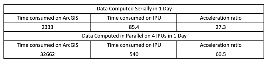
We implemented and accelerated the Kriging algorithm on IPU and achieved excellent results. On IPU-M2000 server, when the number of weather element points is 2167 and the number of prediction points is 7346*4534, the execution efficiency of IPU is 15.7 times higher than ArcGIS. In the case that all the six weather elements (daily average air pressure, average wind speed, average humidity, average temperature, highest temperature and lowest temperature) are calculated at the same time to generate the complete weather forecast map ET₀, the execution efficiency of the IPU-optimised code is 27.3 times higher than ArcGIS. When 4 IPUs are used at the same time to calculate the ET₀ for 14 days, the IPU’s execution efficiency is 60.5 times higher than ArcGIS. The main optimisation process is as below:

KD Tree Optimisation

In PyKrige's open-source algorithm, we learned that the implementation of KD Tree uses a single thread, while IPU has an equivalent to more than 50 server CPU cores. After comprehensive experimentation and testing, we used 8 threads to solve KD Tree which maximised the advantages of IPU parallelism. As a result, the time consumed by KD Tree was reduced from 34 down to 8 seconds.

Interpolation Prediction Optimisation

In PyKrige's open-source algorithm, the vector λ is solved line by line, which requires a total of 7346*4534 executions, and the linear solver speeds at each execution can be very slow. As reference, it takes about 2000 seconds to calculate all the data in the original implementation. Using cython can significantly enhance the calculation efficiency, but it still takes about 300 seconds to match the built-in speed of ArcGIS. We then used TensorFlow to port the solution and point multiplication process to the IPU, and make full use of the IPU’s on-chip memory to perform matrix inversion and point multiplication with a batch size of 20,000. Using the IPU's powerful matrix computing capabilities and large batch processing improved the calculation of the entire dataset from 2000 to 21 seconds.

Pre-processing Optimisation

The original weather element data needs to be pre-processed with IDL software. In order to get performance gains, we have implemented an IDL script that feeds the pre-processing results directly into Kriging interpolation. The whole algorithm is now an end-to-end process with no need to access intermediate calculation results.

Algorithm Flow Optimisation

Meteorological points are consistent every day, so the Euclidean distance calculation and kdtree solution will not change. The results for the six weather elements are completely consistent and would only need to be calculated once so as to optimise our distance algorithm's solution time.

Multi-IPU Parallel Computing

We used 4 IPUs to calculate the interpolation results. The parallelisation greatly improved the operation efficiency, completing the calculation in 4 days.

Summary

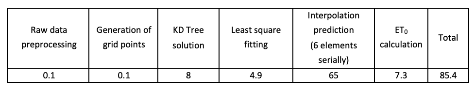
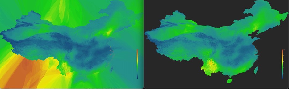
The single-day overall performance of ET₀ calculation in the IPU is shown in Table 2, and the acceleration performance is shown in Table 3. A comparison of the final output results between the IPU and the ArcGIS calculation is shown in Figure 4. Focusing entirely on the image within the map borders, it can be seen that the output of the IPU recursion is comparable to the distribution of weather elements in the map generated by ArcGIS.