Jun 14, 2022
Jun 14, 2022
We're Hiring
Join us and build the next generation AI stack - including silicon, hardware and software - the worldwide standard for AI compute
Join our teamMichael Bronstein is the DeepMind Professor of AI at the University of Oxford and Head of Graph Learning Research at Twitter. A version of this post first appeared on his blog. Professor Bronstein co-authored this post with Emanuele Rossi from Twitter and Daniel Justus from Graphcore.
UPDATE: TGN Training is now available to run as a Paperspace Gradient Notebook.
![]()
Graph-structured data arise in many problems dealing with complex systems of interacting entities. In recent years, methods applying machine learning methods to graph-structured data, in particular Graph Neural Networks (GNNs), have witnessed a vast growth in popularity.
The majority of GNN architectures assume that the graph is fixed. However, this assumption is often too simplistic: since in many applications the underlying system is dynamic, the graph changes over time. This is for example the situation in social networks or recommendation systems, where the graphs describing user interaction with content can change in real-time. Several GNN architectures capable of dealing with dynamic graphs have recently been developed, including our own Temporal Graph Networks (TGNs)[1].
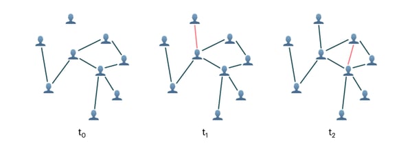
A graph of interactions between people is changing dynamically by gaining new edges at timestamps t1 and t2
In this post, we explore the application of TGNs to dynamic graphs of different sizes and study the computational complexities of this class of models. We use Graphcore’s Bow Intelligence Processing Unit (IPU) to train TGNs and demonstrate why the IPU’s architecture is well-suited to address these complexities, leading to up to an order of magnitude speedup when comparing a single IPU processor to an NVIDIA A100 GPU.
The TGN architecture, described in detail in our previous post, consists of two major components: First, node embeddings are generated via a classical graph neural network architecture, here implemented as a single layer graph attention network[2]. Additionally, TGN keeps a memory summarizing all past interactions of each node. This storage is accessed by sparse read/write operations and updated with new interactions using a Gated Recurrent Network (GRU)[3].
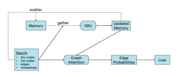
TGN model architecture. Bottom row represents a GNN with a single message passing step. Top row illustrates the additional memory for each node of the graph
We focus on graphs that change over time by gaining new edges. In this case, the memory for a given node contains information on all edges that target this node as well as their respective destination nodes. Through indirect contributions, the memory of a given node can also hold information about nodes further away, thus making additional layers in the graph attention network dispensable.
We first experiment with TGN on the JODIE Wikipedia dataset[4], a bipartite graph of Wikipedia articles and users, where each edge between a user and an article represents an edit of the article by the user. The graph consists of 9,227 nodes (8,227 users and 1,000 articles) and 157,474 time-stamped edges annotated with 172-dimensional LIWC feature vectors[5] describing the edit.
During training, edges are inserted batch-by-batch into the initially disconnected set of nodes, while the model is trained using a contrastive loss of true edges and randomly sampled negative edges. Validation results are reported as the probability of identifying the true edge over a randomly sampled negative edge.
Intuitively, a large batch size has detrimental consequences for training as well as inference: The node memory and the graph connectivity are both only updated after a full batch is processed. Therefore, the later events within one batch might rely on outdated information as they are not aware of earlier events in the batch. Indeed, we observe an adverse effect of large batch sizes on task performance, as shown in the following figure:
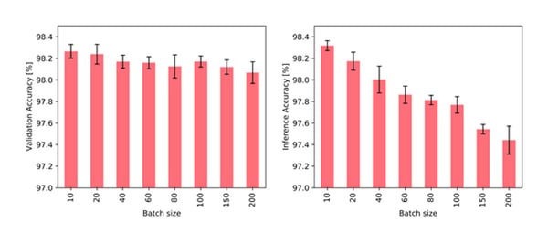
Accuracy of TGN on JODIE/Wikipedia data when training with different batch sizes and validating with a fixed batch size of 10 (left) and when training with a fixed batch size of 10 and validating with different batch sizes (right).
However, the use of small batches emphasizes the importance of fast memory access for achieving a high throughput during training and inference. The IPU with its large In-Processor-Memory, therefore, demonstrates an increasing throughput advantage over GPUs with smaller batch size, as shown in the following figure. In particular, when using a batch size of 10 TGN can be trained on the IPU about 11 times faster, and even with a large batch size of 200 training is still about 3 times faster on the IPU.
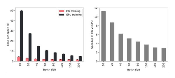
Throughput improvement for different batch sizes when using a single IPU out of a Bow2000 IPU system compared to an NVIDIA A100 GPU.
To better understand the improved throughput of TGN training on Graphcore’s IPU, we investigate the time spent by the different hardware platforms on the key operations of TGN. We find that the time spent on GPU is dominated by the Attention module and the GRU, two operations that are performed more efficiently on the IPU. Moreover, throughout all operations, the IPU handles small batch sizes much more efficiently.
In particular, we observe that the IPU’s advantage grows with smaller and more fragmented memory operations. More generally, we conclude that the IPU architecture shows a significant advantage over GPUs when the compute and memory access are very heterogeneous.
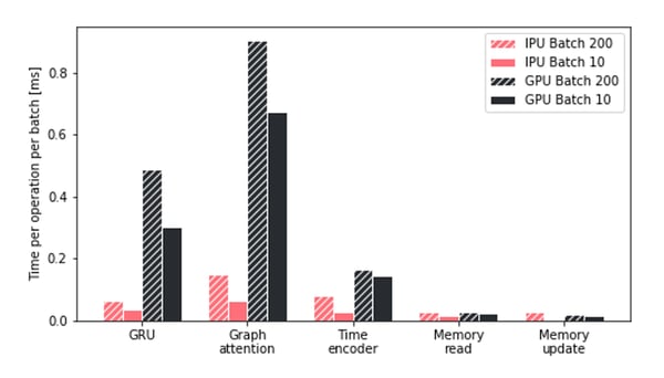
Time comparison for the key operations of TGN on IPU and GPU with different batch sizes.
While the TGN model in its default configuration is relatively lightweight with about 260,000 parameters, when applying the model to large graphs most of the IPU In-Processor-Memory is used by the node memory. However, since it is sparsely accessed, this tensor can be moved to off-chip memory, in which case the In-Processor-Memory utilisation is independent of the size of the graph.
To test the TGN architecture on large graphs, we apply it to an anonymized graph containing 261 million follows between 15.5 million Twitter users[6]. The edges are assigned 728 different time stamps which respect date ordering but do not provide any information about the actual date when follows occurred. Since no node or edge features are present in this dataset, the model relies entirely on the graph topology and temporal evolution to predict new links.
Since the large amount of data makes the task of identifying a positive edge when compared to a single negative sample too simple, we use the Mean Reciprocal Rank (MRR) of the true edge among 1000 randomly sampled negative edges as a validation metric. Moreover, we find that the model performance benefits from a larger hidden size when increasing the dataset size. For the given data we identify a latent size of 256 as the sweet spot between accuracy and throughput.
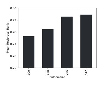
Mean Reciprocal Rank among 1000 negative samples for different hidden sizes of the model.
Using off-chip memory for the node memory reduces throughput by about a factor of two. However, using induced subgraphs of different sizes as well as a synthetic dataset with 10× the number of nodes of the Twitter graph and random connectivity we demonstrate that throughput is almost independent of the size of the graph (see table below). Using this technique on the IPU, TGN can be applied to almost arbitrary graph sizes, only limited by the amount of available host memory while retaining a very high throughput during training and inference.
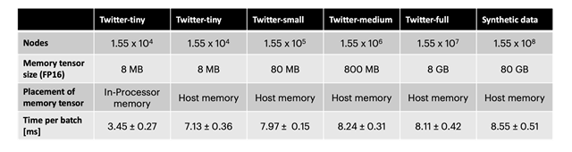
Time per batch of size 256 for training TGN with hidden size 256 on different graph sizes. Twitter-tiny is of a similar size as the JODIE/Wikipedia dataset.
As we have repeatedly noted previously, the choice of hardware for implementing Graph ML models is a crucial, yet often overlooked problem. In the research community, in particular, the availability of cloud computing services abstracting out the underlying hardware leads to certain “laziness” in this regard. However, when it comes to implementing systems working on large-scale datasets with real-time latency requirements, hardware considerations cannot be taken easily anymore. We hope that our study will draw more attention to this important topic and pave the way for future more efficient algorithms and hardware architectures for Graph ML applications.
[1] E. Rossi et al., Temporal graph networks for deep learning on dynamic graphs (2020) arXiv:2006.10637. See accompanying blog post.
[2] P. Veličković, et al., Graph attention networks (2018) ICLR.
[3] K. Cho et al., On the properties of neural machine translation: Encoder-Decoder approaches (2014), arXiv:1409.1259.
[4] S. Kumar et al., Predicting dynamic embedding trajectory in temporal interaction networks (2019) KDD.
[5] J. W. Pennebaker et al., Linguistic inquiry and word count: LIWC 2001 (2001). Mahwah: Lawrence Erlbaum Associates 71.
[6] A. El-Kishky et al., kNN-Embed: Locally smoothed embedding mixtures for multi-interest candidate retrieval (2022) arXiv:2205.06205.
Share: