Apr 17, 2023
Apr 17, 2023
We're Hiring
Join us and build the next generation AI stack - including silicon, hardware and software - the worldwide standard for AI compute
Join our teamIn light of the significant growth in deep learning model size as well as the increased uptake of artificial intelligence across a broad range of applications, the incentives to reduce the computational cost of running these models have never been greater.
One method that has shown significant promise to reduce these costs is to use sparsity. Sparsity typically refers to the method of inducing as many zeros as possible in the model weights through a process of pruning, then skipping these values when doing the computation itself.
While much success has been achieved in using sparsity to reduce theoretical measures of cost like FLOPs and parameter count, achieving actual speed improvements while maintaining acceptable task performance has been much more difficult, particularly on general-purpose accelerators such as GPUs using low-precision number formats.
To help realise these theoretical benefits in practice and enable further investigation of sparse techniques on Graphcore IPUs, we introduce PopSparse, a library that enables fast sparse operations by leveraging both the unique hardware characteristics of IPUs as well as any block structure defined in the data. We target two different types of sparsity: static, where the sparsity pattern is fixed at compile-time; and dynamic, where it can change each time the model is run.
We benchmarked sparse dense matrix multiplication for both modes on IPU.
Results indicate that the PopSparse implementations are faster than dense matrix multiplications on IPU at a range of sparsity levels with large matrix size and block size. Furthermore, static sparsity in general outperforms dynamic sparsity.
While previous work on GPUs has shown speedups only for very high sparsity (typically 99% and above), we demonstrate that Graphcore’s static sparse implementation outperforms equivalent dense calculations in FP16 at lower sparsity (around 90%).
These results were published online on arXiv and accepted to the Sparse Neural Network workshop at ICLR 2023.
The notion of sparsity in deep learning most commonly refers to the idea of sparsifying the model weights with the aim of reducing the associated storage and compute costs. This is typically done through a single pruning step at the end of training (Zhu & Gupta, 2017) or potentially through some sparse training regime (Evci et al., 2019). These approaches have typically achieved between 90–99% reduction in model weights while maintaining and acceptable level of accuracy (Hoefler et al., 2021).
While the benefits to model size can be easily realised, increased computational efficiency can often be more difficult to achieve as the resulting unstructured sparsity patterns do not align well with the vectorised instruction sets in highly parallel deep learning accelerators (Qin et al., 2022). Therefore, one approach to improving sparse compute efficiency is to enforce some degree of structure on the sparsity pattern.
This has motivated a wide range of structured pruning techniques such as neuron (Ebrahimi & Klabjan, 2021), channel-wise (He et al., 2017), block (Gray et al., 2017), 2:4 (Mishra et al., 2021). However, these methods generally incur a task performance penalty compared to equivalent unstructured methods.
Here we present PopSparse, a library for the effective acceleration of sparse dense matrix multiplication (SpMM) on Graphcore IPUs. IPUs have multiple architectural features that help accelerate sparse operations:
The SpMM can be written as:
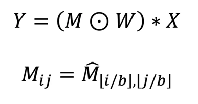
Where ⊙ denotes elementwise multiplication, * for inner product, Y ∈ Rᵐ ˣⁿ, X ∈ Rᵏ ˣⁿ are dense output and input matrices respectively. The sparse weight matrix (M⊙W) is defined via M ∈ Bᵐ ˣᵏ (B = {0,1}), a mask that represents the sparsity pattern, itself derived from M̂ ∈ B⁽ᵐᐟᵇ⁾ˣ⁽ᵏᐟᵇ⁾, a block mask and W ∈ Rᵐ ˣᵏ defines weight values.
In this formulation, (M⊙W) has a block-sparse structure, where contiguous square blocks of weights of shape b × b contain all the non-zero elements, given block-size b. The dimensions m and k are referred to as output and input feature size and n is referred to as batch size, corresponding to their typical role in weight-sparse neural network computation.
We define density, d = ∑ᵢⱼMᵢⱼ/(m⋅k), where the standard term sparsity corresponds to (1 — d). We use floating point operation (FLOP) count to quantify the amount of useful arithmetic work in an SpMM as: 2⋅m⋅k⋅n⋅d. Note that this only counts operations performed on non-zero values and does not depend on block size b. The PopSparse library supports unstructured (block size b = 1) or structured sparsity (b = 4, 8, 16).
With static sparsity, during compile time, the sparsity pattern and matrix shapes are known to the partitioner, which splits the non-zero elements (specific values not known yet) of the sparse matrix across k dimension into qₖ partitions and the dense matrix across n dimension into qₙ partitions.
Figure 1a illustrates the distribution, computation and reduction of the sparse matrix in the static sparse case. Splits over the k dimension do not have to be evenly sized and are chosen to ensure a balanced distribution of the non-zero elements (denoted with coloured small blocks in the figure).
Once the model is compiled, during execution, the specific non-zero values of W are provided. As the sparsity pattern is known in advance, no extra exchange of data is needed. Local dot product computation with the dense matrix is then executed and there is a final reduction across tiles to give the dense output matrix.
With dynamic sparsity, the maximum number of non-zero elements for the sparse operand is fixed, while the sparsity pattern is updated during execution. To minimise compute cycles, we employ a planner during compile time to optimise the partitioning while accommodating for the full range of sparsity patterns that can be defined during execution.
As the sparsity pattern could change for each run, compared to static sparsity, there is an additional step to distribute sparse matrix indices and non-zero values by the partitioner. This is demonstrated in Figure 1b. Furthermore, as fixed size partitions over m and k dimensions are required, the number of non-zero elements in each partition may not be balanced.
In Figure 1b the B elements on the second partition of k dimension do not fit on Tile1. Three of the B elements overflow to Tile2. However, the Tile2 does not have all the partition information (slices of m, k, n) corresponding to B elements to compute the result. Consequently, extra steps of propagation are induced to finish the computation.
Overall, our dynamic sparse implementation has several additional costs compared to the static case:
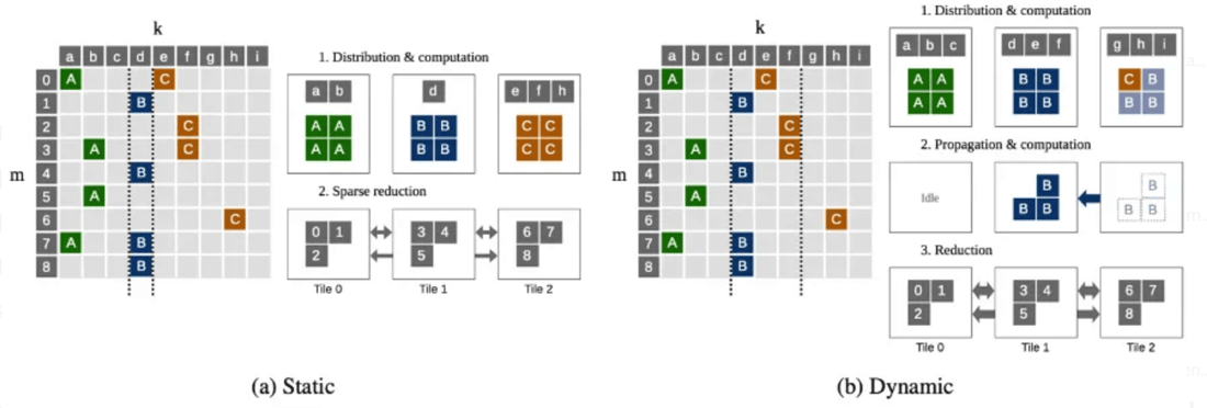
Figure 1: Illustration of static and dynamic sparse partitioning of the input feature dimension, k.
Our micro benchmarking experiments explore a single sparse-dense matmul SpMM: Y=(M⊙W)*X on IPU and GPU. The APIs used for IPU experiments and GPU baselines are shown in Table 1. The range of parameters that were benchmarked is detailed in Table 2.
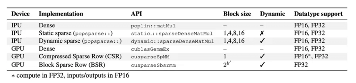
Table 1: APIs used when benchmarking IPU and GPU.
IPU: The operation is executed a single time on a single Bow IPU in a Bow-2000 chassis, with a randomly generated sparsity pattern and values. We extract cycle count information and convert these cycle counts into TFLOP/s values given a constant clock of 1.85 GHz. Host transfers are excluded from measured time.
GPU: Baseline sparse implementations on GPU are provided by the cuSPARSE library v11.6.2 (NVIDIA, 2022). These are divided according to the sparse format used, with no distinction between static and dynamic sparsity patterns. We consider compressed sparse row (CSR) and block sparse row (BSR) for unstructured and block sparsity, respectively. We generate a random sparsity pattern and values, copy to device, execute 25 iterations of the operation and copy results to host for validation. We start timing after 5 iterations and measure wall clock time using cudaEventRecord. All experiments were performed on a single A100 GPU running in a 4 x A100-SXM4–40G chassis.
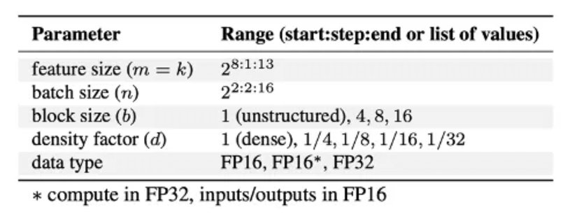
Table 2: Ranges of parameters swept for benchmarks.
The key results of this work are shown in Figure 2. These plots show the compute FLOP/s (in log scale) vs density with fixed feature size, with each line presenting different implementations of the same operation. By construction, the dense implementation shows linear scaling with density — since zeros are not counted in the FLOP/s calculation. While on the other hand, for a sparse implementation, perfect scaling would predict constant FLOP/s as density varies.
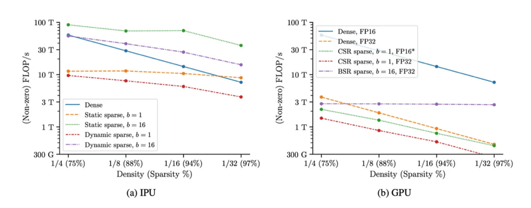
Figure 2: IPU FP16 and GPU block-sparse matmul performance as density varies for various block size b, square feature size m = k = 4096, best over batch size n.
For the dense baselines, while we broadly see chip-for-chip parity between IPU and GPU in FP16, it's important to highlight that the IPUs used are approximately half the price in the cloud, highlighting their cost efficiency for these basic operations. Furthermore, for the sparse operations, we see even larger benefits from using IPUs.
Specifically, for IPUs (Figure 2a), we see that using static sparse operations and block sparsity both individually improve performance. For example, the block size 16, dynamic case shows benefits over the dense baseline across all densities considered and unstructured (b = 1) static sparsity outperforming dense in the low-density regime (<5%). In addition, when both static and block sparsity methods are used, we see benefits of as much as 5x in throughput over the dense baseline.
For the GPU (Figure 2b), we see much less favourable performance with the sparse operations, with no case tested outperforming the FP16 dense baseline. However, we did find that the FP32 block sparse (BSR) case scaled very well as density decreased. It looks possible that for very low densities, this may outperform the dense baseline.
Comparing the two platforms, we can therefore see that IPUs achieve as much as a 5x throughput benefit over the dense GPU baseline and as much as a 25x throughput improvement when only sparse operations are considered. With the additional price benefits, we believe this presents a compelling case for investigating sparse applications on IPUs.
It should however be noted that even on IPU, the sparse operations only outperform the dense baselines under certain conditions. More extensive result can be found in our paper, but as an approximate guide, sparsity typically brings speedup over the dense baseline on IPU (FP16, large batch size for both) when:
Try PyG on IPUs for free
![]()
[1] Michael Zhu and Suyog Gupta. To prune, or not to prune: exploring the efficacy of pruning for model compression, 2017. URL https://arxiv.org/abs/1710.01878.
[2] Utku Evci, Trevor Gale, Jacob Menick, Pablo Samuel Castro, and Erich Elsen. Rigging the lottery: Making all tickets winners, 2019. URL https://arxiv.org/abs/1911.11134.
[3] Torsten Hoefler, Dan Alistarh, Tal Ben-Nun, Nikoli Dryden, and Alexandra Peste. Sparsity in deep learning: Pruning and growth for efficient inference and training in neural networks, 2021. URL https://arxiv.org/abs/2102.00554.
[4] Eric Qin, Raveesh Garg, Abhimanyu Bambhaniya, Michael Pellauer, Angshuman Parashar, Sivasankaran Rajamanickam, Cong Hao, and Tushar Krishna. Enabling flexibility for sparse tensor acceleration via heterogeneity, 2022. URL https://arxiv.org/abs/2201.08916.
[5] Abdolghani Ebrahimi and Diego Klabjan. Neuron-based pruning of deep neural networks with better generalization using kronecker factored curvature approximation, 2021. URL https://arxiv.org/abs/2111.08577.
[6] Yihui He, Xiangyu Zhang, and Jian Sun. Channel pruning for accelerating very deep neural networks, 2017. URL https://arxiv.org/abs/1707.06168.
[7] Scott Gray, Alec Radford, and Diederik P. Kingma. GPU kernels for block-sparse weights. 2017.
[8] Asit Mishra, Jorge Albericio Latorre, Jeff Pool, Darko Stosic, Dusan Stosic, Ganesh Venkatesh, Chong Yu, and Paulius Micikevicius. Accelerating sparse deep neural networks, 2021. URL https://arxiv.org/abs/2104.08378.
[9] NVIDIA. API reference guide for cuSPARSE, 2022. URL https://docs.nvidia.com/cuda/cusparse/.
This article was originally published in Towards Data Science.
Share: