Fine-tune GPT-J: a cost-effective GPT-4 alternative for many NLP tasks

Updated July 2023: speeding-up GPT-J using Group Quantisation

It's clear that hot new generative AI models like ChatGPT, GPT-3 and GPT-4 can produce astounding results. But do we really need models of this size for every language application, or can we achieve state-of-the-art performance for many NLP tasks with a smaller model, like GPT-J? 

The answer is yes. For downstream tasks such as Question Answering, Named Entity Recognition, Sentiment Analysis, and Text Classification, smaller models can easily be fine-tuned to deliver SOTA results. Larger models mainly add more world knowledge and better performance at free text generation as might be used in an AI Assistant or chatbot.  

OpenAI does not make the trained weights for GPT-4, GPT-3 or ChatGPT freely available, and training models on this scale from scratch is prohibitively expensive. The company does offer limited fine-tuning as-a-service, but users are required to share their training data, pay for the fine-tuning process, and pay on an ongoing basis to access the resulting model.

For many companies, choosing a more efficient, highly performant smaller model, like GPT-J, is the right choice. 

GPT-J is an open-source alternative to OpenAI's GPT-3 from EleutherAI. It’s a 6B parameter version of GPT-3 that anyone can download and which performs just as well as larger models on many language tasks. 

GPT-J is available to run today - both for inference and fine-tuning - on Graphcore IPUs, using Paperspace Gradient Notebooks. Inference can be run on any system from IPU-Pod₄ upwards.

In this blog post and accompanying video tutorial, we will show you how to fine-tune a pretrained GPT-J model in an easy to use Jupyter notebook on Paperspace, running on a 16 IPU system. It takes around 2 hours 47 minutes to run through this notebook in its entirety on the Bow Pod₁₆ platform and faster if you want to run it on a larger system in production.

We will explain how you can fine-tune GPT-J for Text Entailment on the GLUE MNLI dataset to reach SOTA performance, whilst being much more cost-effective than its larger cousins. 

We formulate the MNLI task as a text-to-text problem using stylized prompts. This approach, first presented in the paper 'Exploring the limits of transfer learning with a unified text-to-text transformer', is very general and can be used to fine-tune GPT-J or other generative models out-of-the-box on every down-stream task. 

The strength of this technique is that you can use the same model architecture and pre-trained starting point for many different tasks. The specificity of the down-stream task is captured in the prompt format and during fine-tuning the model learns to associate the given format with the task. 

Crucially, all the language understanding capabilities needed to solve the task are already present in the pre-trained model. Fine-tuning is needed just to learn the prompt-to-task association and is thus relatively cheap.  

An overview of causal decoder-only models 

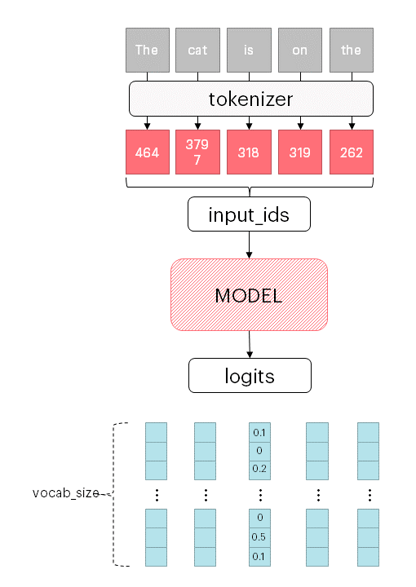
The first step in every language model is tokenization. Tokenizing a text means splitting it into pieces, the tokens, which can be words or sub-words, depending on the tokenizer. Tokens are then converted to ids via a table look-up. The size of such a table is the vocabulary size. 

Details of the tokenization process are important to understand how sensitive a given model is to changes in the input text. 

At the higher level, an autoregressive causal model is a black box that takes a tokenized input sentence and, for each token, outputs the probability distribution for the next token, conditioned on the past tokens. More precisely, it outputs the non-normalised probabilities, the logits. It is understood that when a real probability distribution is needed logits are normalised via a softmax function.

Put simply, the model outputs a vector of size vocab_size for each token, whose component i represents how likely is token i to be the next token, given the previous tokens in the sentence. 

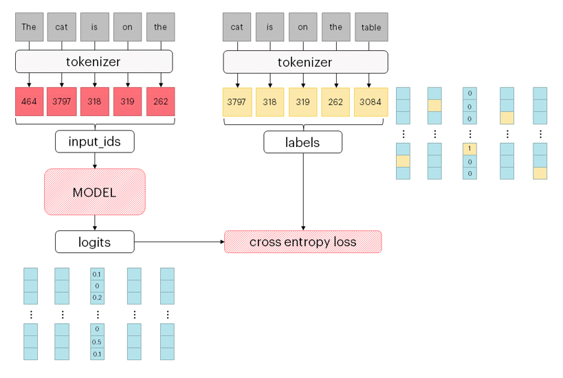
At training time, the shifted input sentence is provided as labels for the model. Implicitly, labels define the target distribution as a categorical distribution where a single class has probability 1 and all the others are 0: basically, target vectors are one-hot encoded vectors. 

The cross entropy loss is used during training to measure the “distance” between these two distributions: the model output distribution and the target one. 

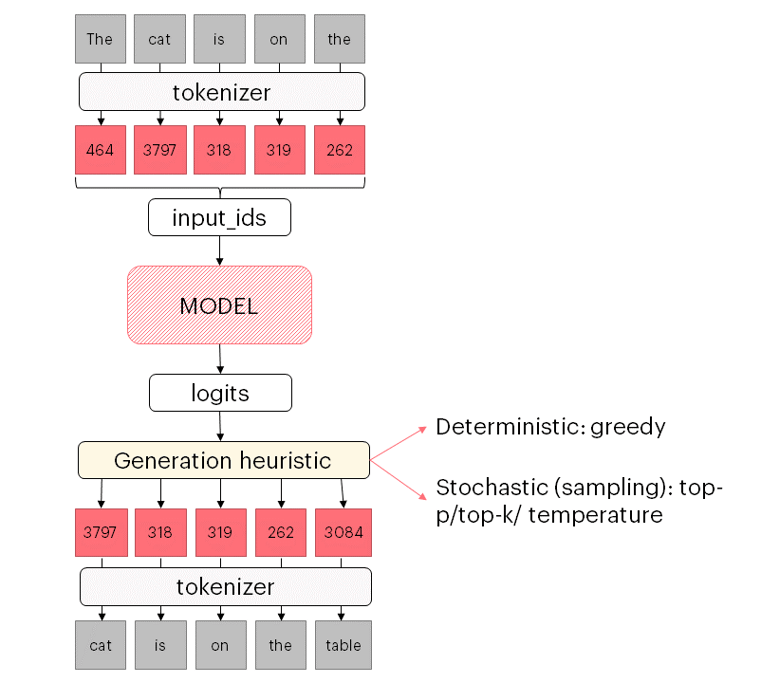
At inference time, logits are instead used to predict the next token following a chosen heuristic (for a nice summary, see this Hugging Face blog post). The simplest case is a greedy heuristic, where next token is selected picking the one corresponding to the highest logits. 

GPT-J MNLI fine-tuning 

With this background, you are equipped to understand the basic functioning of GPT-J fine-tuning. 

Let’s dive into the MNLI example. For a line-by-line explanation you can check out our video walkthrough, where we also explain how to run it in Paperspace.

1. Dataset pre-processing — Cast the task to text-to-text format 

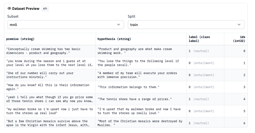
The MNLI dataset consists of pairs of sentences, a premise and a hypothesis. The task is to predict the relation between the premise and the hypothesis, which can be:

• entailment: the premise entails the hypothesis
• contradiction: hypothesis contradicts the premise
• neutral: hypothesis and premise are unrelated.

You can explore the dataset on Hugging Face:

To cast the task into a text-to-text format, we can form training prompts: 
The tokenized prompts provide the inputs and labels for fine-tuning. Since the model is asked to predict the next token, the input consists of the full tokenized sentence but for the last token (prompt[:-1]), and the label is the tokenized sentence shifted by one (prompt[1:]). 

In fact, different sentences are grouped together up to the model sequence length. Given the causal nature of the model, no extra care is needed to separate the sentences (we don’t need a mask). Input and labels are extracted from the packed sentences. 

A similar pre-processing is done also on the validation split of the dataset. 

2. Customise configuration

Once dataset pre-processing is completed, we can customise the training and validation configuration. 

For training, we can customise the optimiser parameters, dropout probability, the number of training steps and parameters controlling checkpoint periodicity. 

For validation, we typically want to control the maximum allowed output tokens, shrink the sequence length and increase the batch size. Moreover, we need to define a metric to measure the model performance. For MNLI, accuracy is used.

3. Instantiate a GPTJTrainer

Finally, we define the pre-trained model. This is the EleutherAI base checkpoint available on Hugging Face. These weights are the starting point for our fine-tuning. 

pretrained = GPTJForCasualLM.from_pretrained(r"EleutherAI/gpt-j-6B")

All these ingredients are used to create a GPTJTrainer: 

trainer = GPTJTrainer(
   config,
   pretrained,
   dataset,
   eval_dataset,
   eval_config,
   tokenizer,
   accuracy_metric,
   postprocess_mnli_predictions,
)

4. Run fine-tuning

With the GPTJTrainer we can run fine-tuning with a single command 

trainer.train()

5. Run validation

Validation is just as easy: 

trainer.evaluate()

6. Convert to HF checkpoint

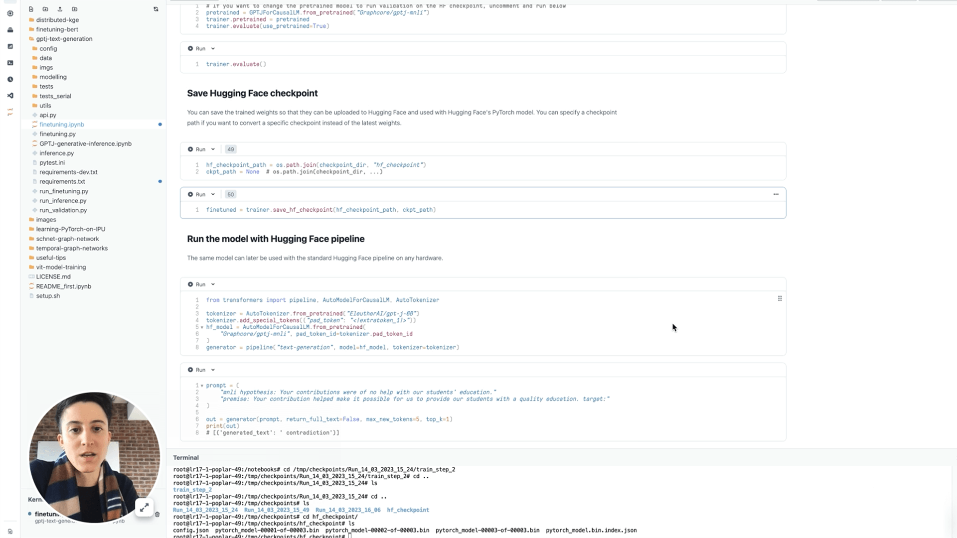
Once we have fine-tuned the model and validated it, we can save a Hugging Face compatible checkpoint which can later be uploaded to the HUB. 

finetuned = trainer.save_hf_checkpoint(hf_checkpoint_path, ckpt_path)

Group Quantisation

For large language model generative inference – and this includes GPT-J, the time it takes to generate each token is typically limited by the rate at which weights can be loaded from SDRAM rather than the compute time. 

One strategy for increasing speed is Group Quantisation. Here instead of weights being stored in SDRAM verbatim, they are stored compressed. A common scheme is to divide each weights matrix into groups of 64 elements and for each group store the maximum and minimum values as FP16, divide the range between min and max into 16 intervals and code individual elements as an INT4 by the interval that they fall into. This gives a compression of about 3.5x. There is a small loss of accuracy for using these compressed values, but it is typically only about a percent. With GPT-J, using this approach gives a 2.5x speed-up. 

There is a Paperspace notebook exploring Group Quantisation and showing how it works with GPT-J.

Conclusion

GPT-J is easy to access on IPUs on Paperspace and it can be handy tool for a lot of applications. This notebook runs on a 16 IPU instance from Graphcore (Pod16), which is a low cost cloud instance and is the best starting point for GPT-J exploration.

For higher performance and faster results in production, we would recommend using a 64 IPU cloud instance (you guessed it, Pod64) which is coming soon on Paperspace.

If you would like to be notified when Pod64 systems are available on Paperspace, please join the waiting list here.