PackedBERT: How to accelerate NLP tasks for Transformers with packing

As large language models (LLMs) like the GPT (Generative pre-trained transformer) family capture the public imagination, the practicality of smaller Transformer models like BERT should not be underestimated. While language understanding tasks may work well with models like GPT, it is usually faster and cheaper to use smaller models like BERT, which give you the same or better performance, because they are trained specifically for focused language understanding tasks, while using much less compute and energy.

At Graphcore, we have recently worked on advancing a method called packing for fine-tuning and inference to optimise natural language processing (NLP) models at the application level. This blog post will explain the concept of packing for fine-tuning NLP tasks, and show you how to use it with easy-to-use utilities for Hugging Face on IPUs.

Graphcore customer, Pienso, uses this technique in their production text analytics and insight platform, which you can read about in an earlier blog post, "How Graphcore's BERT breakthrough made Pienso's LLM more efficient".

Why do we want to speed up narrow tasks?

Packing is particularly beneficial for creating solutions that are online-capable, meaning they:

• Scale well
• Handle large incoming loads of data well
• Consume less compute with no performance degradation
• Reduce the overall time of fine-tuning/inference tasks

The technique is both throughput focused and aims to reduce as much computational waste as possible to improve efficiency. It works well with increasing scale — creating large effective increases in batch size with negligible overhead, making it useful for production as well as as research tasks.

As an example, implementing packing for multi-label classification with the GoEmotions dataset showed a 6x speedup for fine-tuning and a 9x speedup for inference workloads, bringing model processing to near real-time speeds!

Note that packing is not specific to BERT and is in theory applicable to any model which processes data on a token-by-token basis with none or minimal cross-token interaction. It can potentially also be applied to genomics and protein folding models, and other transformer models. It is worth noting, however, that its applicability is dependent on the structure of the dataset used, as described in the next section.

This implementation for fine-tuning and inference tasks was inspired by and builds on the work done to create Packed BERT for pre-training.

What is packing?

Put simply, packing as a concept for LLM inputs means to concatenate multiple tokenized sequences together into a single input, which we can call a ‘pack’.

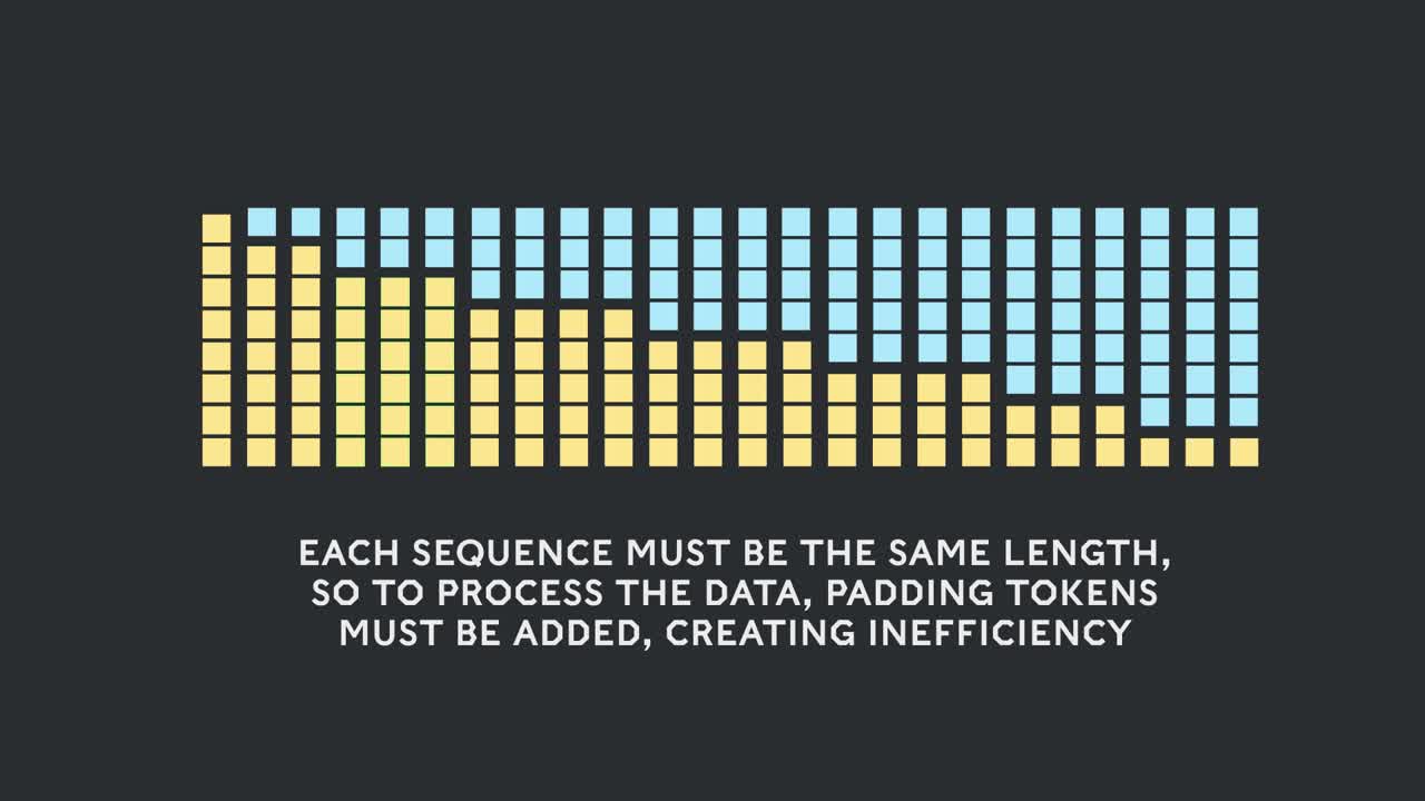
A surprising amount of datasets contain heavily skewed length distributions towards the shorter side, and transformer models receive fixed sized inputs. This is often handled by simply padding the part of the input that isn’t used by the sequence with unused values.

Packing sequences together works to eliminate padding, exploiting the unused space to mitigate computational waste, while maintaining the benefits of a model represented as a static graph with constant-sized inputs. It also means more sequences are being processed per batch, with multiple sequences (within a pack) being processed in parallel on a token level. This effectively increases batch size, with minimal overhead, and brings with it massive throughput benefits.

Dataset length distributions

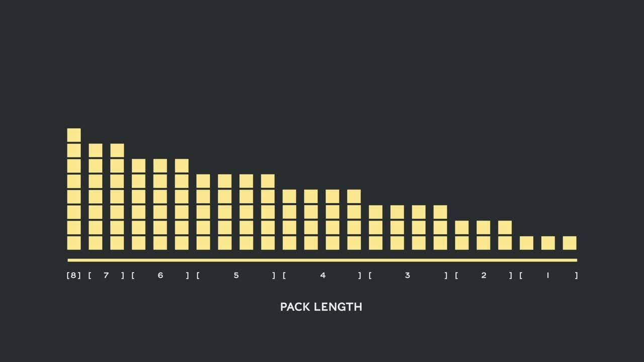
The time-optimisation that packing provides relies on datasets with sequence length distributions which are skewed to the shorter side of the maximum sequence length. It works by fitting multiple sequences into one sample, essentially treating each sample as a batch within a batch.

For training, increasing effective batch size in this way means further hyperparameter tuning is needed. For inference, since hyperparameter consideration is not needed, even higher throughput can be theoretically achieved.

The code walkthrough in this article demonstrates a 9x speed-up for inference and 6x speedup for training.

For perspective, we undertook a brief analysis of the dataset characteristics of some of the most popular fine-tuning text classification datasets on Hugging Face Hub, based on number of downloads. The pool contains 10 of the most popular datasets, with most subsets included, barring a couple which were prohibitively large relative to others. In total, this makes up 39 datasets.

These datasets were tokenized to an arbitrary short sequence length of 256 and manually generated by extracting only the list of sequence lengths for each sample in the dataset. These sequence lengths were used to create a length distribution histogram from 0 to 256 with a bin size of 5:

Observing this histogram, it is apparent that there is a strong skew towards shorter length sequences in the majority of the datasets, with a small number of components at longer lengths, constituted mostly by datasets which focus on long contexts.

Why does packing work with language models like BERT?

BERT is an encoder heavy natural language model commonly used for language analysis and prediction tasks. Text samples are passed to BERT after being tokenized (mapped to a word-specific integer value that corresponds to the model vocabulary). For BERT, each sequence of tokens is processed in parallel, on a token-by-token basis, with positional, syntactic and semantic information about the token encoded within the sample’s embeddings, which are learned over each sequence through the Transformer multi-headed self-attention mechanism.

This is incredibly useful, it means that in theory, individual token information can be analysed with respect to the sequence it is part of, without interference from other sequences passed within the input. This behaviour is already exhibited by transformers in datasets which contain more than one sentence being part of a single input sequence.

A key element of transformers is the attention mask, which allows the self attention to concentrate its context oriented token-specific learning to a particular part of the sequence.

This allows us to pack an input with multiple sequences to achieve the desired throughput benefit. In practice, there are a few tweaks to make to the model, particularly at the output stage, in order to be able to perform classification and prediction tasks with packed inputs. Take a look at the diagram below for a straightforward visualisation of how we can pack multiple sequences to mitigate computational waste from padding and speed up the model, as compared to BERT without packing:

There are essentially 3 stages to packing, particularly for fine-tuning:

• An algorithm that is as fast as possible at packing as many sequences as possible together, as close to optimally as possible.
• Adjusting the model’s input to interpret a single input as multiple sequences rather than a single sequence and padding using the attention mask.
• Adjusting the model’s output to unravel the packed input back into separate sequences for final cross-token calculations, such as the loss.

The packing algorithm

There are three algorithms outlined for the original packing implementation for pre-training, these are:

• Non-negative least squares histogram packing (NNLSHP)
• Shortest-pack-first histogram packing (SPFHP)
• Longest-pack-first histogram packing (LPFHP)

These algorithms use the sequence length histogram to try to optimally create packs of sequences with varying lengths to minimise the total number of packs (inputs to the model).

In previous implementations for large dataset pre-training, the most optimal possible configuration of lengths was achieved using NNLSHP. This algorithm is explained neatly in the original article:

“The tricky part was the strategy matrix. Each column has a maximum sum of three and encodes which sequences get packed together to exactly match the desired total length; 512 in our case. The rows encode each of the potential combinations to reach a length the total length. The strategy vector x is what we were looking for, which describes how often we choose whichever of the 20k combinations. Interestingly, only around 600 combinations were selected at the end. To get an exact solution, the strategy counts in x would have to be positive integers, but we realised that an approximate rounded solution with just non-negative x was sufficient. For an approximate solution, a simple out-of-the-box solver could be used to get a result within 30 seconds.”

The disadvantages of this approach are that it:

• Significantly increases in complexity for a sequences-per-pack value greater than 3.
• 3 sequences at most per pack in up to 30 seconds is reasonable for pre-training, but for online-capable tasks, and smaller dataset fine-tuning and inference, this can be far too long — especially when entire training runs can be completed in a matter of seconds.

Skewed distributions in small fine-tuning datasets allow packing many more sequences per pack, which is unfeasible with NNLSHP, so lets take a look at a simpler and more adaptive algorithm: SPFHP.

SPFHP scales very well to increasing number of sequences per pack. It operates on a sorted histogram of lengths from longest to shortest and simply looks at each sequence, and checks whether it fits into any pack. If it fits into one pack, it will be placed in that pack — not considering any future sequences — and if it fits into multiple, it will be placed into the pack with the shortest sequence length.

It is more appropriate for small to medium sized datasets and its complexity is not increased by increasing the number of packs. It solves for any given dataset in almost constant time, taking under 0.02 seconds for up to 16 million samples. The complexity of SPFHP increases with sequence length rather than dataset size or sequences-per-pack, so it remains relatively constant for different dataset sizes!

LPFHP is a shortest-to-longest variant of SPFHP, splitting counts to get more ideal fits. In some cases, it can be useful to approach the task longest-pack-first, offering a slightly more optimal fit.

The packing utilities created for the Packed BERT Hugging Face notebooks allows one of SPFHP or LPFHP to be used, to mitigate the potential preprocessing bottleneck of using NNLSHP.

The original algorithm code for all packing algorithms is available in the blogs code.

Implementing packing for BERT fine-tuning with Hugging Face

Have a go at using packing to speed up BERT for multi-label sequence classification yourself: In this section, we’ll look at how to easily use packing with BERT using HuggingFace on the GoEmotions dataset.

You can follow this walkthrough with some visualisation and further explanation by running it in a Paperspace Gradient notebook — all of the code used in this article is available in the multi-label text classification notebook.

The in-depth walkthrough available on Github explains the internal functionality of the high-level functions that make packing so easy to use in Hugging Face. Full explanations of these and the intrinsic details that you might require if you wish to apply packing to your own model/task are provided in that walkthrough.

The GoEmotions dataset is ideal to try fine-tuning for packing as it has an extremely strong sequence length skew towards shorter sequences, and will provide large throughput increases, as the sequence length distribution for it shows:

About the dataset: GoEmotions is a multi-label sentiment analysis dataset, containing approximately 58000 carefully curated comments labeled for 28 categories of emotion, including a ‘neutral’ category. We will train for all labels using one-hot encoding to represent multi-label outputs.

This dataset is easily downloadable during this walkthrough using the datasets library from Hugging Face, which lets you download the processed and ready-to-use dataset from the Hugging Face Hub, so there is no need to download and set up the dataset yourself.

Setting up your environment

First, set up your environment by installing all of the required pip packages for this walkthrough. If you are trying this walkthrough in Paperspace, ensure you are in the Hugging Face Transformers on IPU (Optimum Graphcore) environment, where you can access the packing utilities from the packed-bert folder. The notebooks for packing already have the utilities accessible, but if you are trying this in a separate personal environment, be sure to clone the repository with:

git clone git@github.com:huggingface/optimum-graphcore.git

And navigate to notebooks/packed-bert to be able to use the models, utils and pipeline functionalities.

pip install git+https://github.com/huggingface/optimum-graphcore.git
pip install scikit-learn;
pip install datasets
pip install evaluate
pip install tokenizers
pip install matplotlib
pip install scipy
pip install huggingface_hub;

We will first import the packages we need as well as the packing specific model for sequence classification, and the inference pipeline.

import transformers
import optimum.graphcore
import torch
import numpy as np
import evaluate
from datasets import load_dataset
from transformers import AutoConfig
from huggingface_hub import notebook_login
from transformers import AutoTokenizer
from optimum.graphcore import IPUConfig, IPUTrainer, IPUTrainingArguments
from models.modeling_bert_packed import PipelinedPackedBertForSequenceClassification
from pipeline.packed_bert import PackedBertTextClassificationPipeline
from utils.packing.dataset_creator import PackedDatasetCreator

Next, we define some generic parameters for the walkthrough:

task = "sst2"
model_checkpoint = "bert-base-uncased"
ipu_config_name = "Graphcore/bert-base-uncased"
micro_batch_size = 2
gradient_accumulation_steps = 32
device_iterations = 32
max_seq_length = 256
pod_type = os.getenv("GRAPHCORE_POD_TYPE", "pod4")
executable_cache_dir = os.getenv("POPLAR_EXECUTABLE_CACHE_DIR", "./exe_cache/") + "/packed_bert_slseqcls/"

The task is go_emotions, the checkpoint is the default bert-base-uncased which we will use as a base to fine-tune the model for go_emotions. This model will run on Graphcore IPUs, and to take advantage of the parallelism available on an IPU, we need to define some IPU-specific configurations, from the perspective of fine-tuning, these effectively create a larger batch size for the model.

max_seq_length is the maximum length all input sequences are fixed to, and all sequences below this length will be padded to this length. Given the small size of the sequences in the GoEmotions dataset, we can reduce the model maximum input size to max_seq_length = 256.

IPU Parallelism: We are using both data parallelism and pipeline parallelism (see this tutorial for more). Therefore the global batch size, which is the actual number of samples used for the weight update, is determined using four factors:

global_batch_size = micro_batch_size * gradient_accumulation_steps * device_iterations * replication_factor

We define the gradient accumulation steps, device iterations and micro-batch size. The replication factor (which replicates the model over multiple sets of IPUs) is set to 1 by default, and this walkthrough will use 4 IPUs for a single replica by default. The ipu_config is a special configuration available within all checkpoints in the Graphcore space on the Hugging Face Hub. It contains the defaults for these IPU-specific parameters for the base checkpoint, and must be passed to an IPU-specific model to instantiate it.

Getting and preparing the dataset

To retrieve the dataset, we can simply use load_dataset from the Datasets library, which will retrieve it from the Hugging Face Hub and load it into your script.

We also want to initialise the metric for validating the dataset, since this is a multi-label task with one-hot encoded outputs, we will use the ROC-AUC metric, a common performance measure for multi-class, multi-label classification problems. We can load this from Hugging Face’s Evaluate library.

For preprocessing the model and turning our strings of sentences into integer tokens that correspond to the vocabulary interpreted by BERT, we also need to initialise a model tokenizer. This will convert individual words/sub-words into tokens.

This is easily done using the AutoTokenizer from the Transformers library. The default pre-trained BERT checkpoint contains a pre-configured tokenizer, so we can load the tokenizer with the pre-trained embeddings and vocabulary directly for our model using from_pretrained.

dataset = load_dataset(task)
metric = evaluate.load("roc_auc", "multilabel")
 
tokenizer = AutoTokenizer.from_pretrained(model_checkpoint, use_fast=True)

The map function available in the Datasets library can be used to tokenize the dataset.

First, create a simple function which applies the tokenizer to one text sample, for which we: 

• Define the maximum sequence length
• Set truncation to True: This will truncate any sequences which are larger than the maximum sequence length. 
• Note that for packing, we do not set padding to be true at this stage. We will pad the dataset when we pack it, but packing requires its inputs to be unpadded initially.

Second, we need to encode our labels in the one-hot format. As the dataset allows multiple labels to be true for one input, to keep a constant label dimension, we need to encode the label column in the dataset as a binary array rather than dynamic-length lists of integers representing the label classes. Since there are 28 classes, an example would look like this:

Original labels: [3, 27] 
One hot encoded labels: [0, 0, 0, 1, 0, 0, 0, 0, 0, 0, 0, 0, 0, 0, 0, 0, 0, 0, 0, 0, 0, 0, 0, 0, 0, 0, 0, 1]

Here, 3 and 27 are valid labels for a given input. In the one-hot encoded format, index 3 and index 27 are set to 1 to define this, allowing the valid labels to be of any size.

We wrap the call to tokenize one sample in the first function, and wrap the call to convert one set of labels to a one-hot encoded format in the second function. Then we use the map function to iteratively apply preprocessing to every sample, using internal batching to speed it up, set with the batched argument.

#Tokenising function for one sample
def preprocess_function(examples):
 return tokenizer(
 examples['sentence'], truncation=True, max_length=max_seq_length)

#Label ID to one-hot-encoded conversion for one sample
def id_to_N_hot(example):
 indexes = example['labels']
 label = np.zeros((num_labels,), dtype=np.float16)
 for idx in indexes:
 label[idx] = 1
 example['labels'] = label
 return example

# Call to map the data
encoded_dataset = dataset.map(id_to_N_hot)
encoded_dataset = encoded_dataset.map(preprocess_function, batched=True)

Packing the dataset

Now that we have a preprocessed and tokenized dataset, we can pack the dataset. To summarise what we need to do for packing, there are four steps to ensuring we can use a packed dataset for a model:

1. Create a histogram of the sequence lengths of the dataset.
2. Generate a set of ‘strategies’ for the dataset using one of the state-of-the-art packing algorithms, which map out the order and indices of the sequences that need to be packed together. 
3. Use this strategy to create the actual dataset, concatenating the tokenized features together for each column in the dataset, including the labels.
4. Finally, pass these new columns into a custom PyTorch dataset, ready to be passed to the dataloader!

What is a strategy? The ‘mapping of the order of sequences’ uses the histogram of sequence lengths to group together length values that best fit into a give maximum length. The set of strategies for a dataset contains multiple lists of lengths, covering all of the sequences in the dataset, for instance:

The first strategy in the set of strategies may be [120,40,40,60] indicating one sequence of length 120, two sequences of length 40 and one sequence of length 60 should be placed in the given order to form one pack. There may be multiple sequences with these lengths, so when forming one pack, we can mark a sequence as being ‘used’ to ensure sequence retrieval is not repeated.

The above steps have been simplified through the easy-to-use utils.packing available in the Graphcore Hugging Face repo. We can simply generate the packed dataset after the usual tokenization and preprocessing by passing all necessary packing configuration to the PackedDatasetCreator class, and generate the ready-to-use dataset with .create().

This completes all three of the above steps, and creates the PyTorch dataset.

First, we define some essential packing parameters:

max_seq_per_pack = 6
num_labels = 2
problem_type = 'single_label_classification'

The max_seq_per_pack is the maximum number of sequences that can be concatenated into one input, called a ‘pack’. This effects the overall batch size of the data at the classification stage, and as a result, too large of a value for fine-tuning may result in needing more extensive hyperparameter tuning to get the best results possible.

We have decided to keep the default value at 6 for the current examples, meaning a theoretical speed-up of up to 6 times the speed of an unpacked dataset. For inference, this can be set higher, to get even more throughput for large batched inference workloads.

The PackedDatasetCreator provides quite a few options to modify the process according to the dataset:

• Adjustable maximum sequence length. 
• Adjustable number of sequences per pack max_seq_per_pack .
• The packing algorithm to use (one of LPFHP or SPFHP).
• A custom label key to allow the class to access the labels in the dataset, as these are not tokenized. 
• Currently, the creator class supports single and multi-label classification, and question answering. The type of task is defined using the problem_type, one of single_label_classification, multi_label_classification or question answering. 
• For different tasks, you can set training=True, validation=True or inference=True.

The PackedDatasetCreator class also has some other features specifically for inference, such as pad_to_global_batch_size, a feature useful for performing batched inference on a large samples when we do not want to lose any of the samples when creating data iterators, it applies ‘vertical’ padding to the dataset, adding filler rows to bring the dataset up to a value divisible by the global batch size, and allows for the largest possible batch sizes to be used without any loss of data.

Once the packer has been created (has generated the histogram and packing strategy — the 1st and 2nd steps), we can simply call the .create() which will return fully packed versions of the initial tokenized un-packed datasets, this will perform the 3rd and 4th step of packing the dataset.

train_data_packer = PackedDatasetCreator(
 tokenized_dataset = encoded_dataset['train'],
 max_sequence_length = max_seq_length,
 max_sequences_per_pack = max_seq_per_pack,
 training = True,
 num_labels = num_labels,
 problem_type = problem_type,
 algorithm = 'SPFHP',
 custom_label_key = 'label'
)

val_data_packer = PackedDatasetCreator(
 tokenized_dataset = encoded_dataset['validation'],
 max_sequence_length = max_seq_length,
 max_sequences_per_pack = max_seq_per_pack,
 validation = True,
 num_labels = num_labels,
 problem_type = problem_type,
 algorithm = 'SPFHP',
 custom_label_key = 'label'
)

packed_train_dataset = train_data_packer.create()
packed_val_dataset = val_data_packer.create()

We can then observe the output of the dataset creation, which will show us what packing has actually accomplished here:

Packing efficiency (fraction of real tokens): 42.5296
 Speed-up theoretical limit: 13.3547
 Achieved speed-up over un-packed dataset: 5.67971
 Runtime: Packed 43410 sequences in 0.001 seconds
 Average packing factor: 5.6797069213659555
Packing efficiency (fraction of real tokens): 43.7226
 Speed-up theoretical limit: 13.3873
 Achieved speed-up over un-packed dataset: 5.85329
 Runtime: Packed 5426 sequences in 0.001 seconds
 Average packing factor: 5.853290183387271

Packed dataset creation time: 1.9252s
Packed dataset creation time: 0.1407s

The output shows a theoretically achieved 5.68 times speed up over the unpacked dataset. The algorithm is fast, completing the strategy for all 43410 training sequences in 0.001 seconds. The full process of creating the dataset takes a few seconds, effectively negligible overhead mitigated by the training speed-up.

Observing the packed dataset

Lets have a look at what the columns in the packed dataset look like, to dig a little deeper into what the PackedDatasetCreator has done with the original dataset. 

Within the function, it expects the default column names generated by the tokenizer, specifically: 

• input_ids
• attention_mask 
• labels (for training, validation)
• token_type_ids (optional)

It also generates some extra columns:

• position_ids is a column denoting the position of individual tokens within their respective sequence inside a pack. 
• example_ids (for inference) are integer indices corresponding to the position of a sample within the input data, and are used to re-order inference data outputs to be the same order as the inputs. This is required as the one-time shuffling of the data is a necessary side-effect of packing, in order to reduce the dataset size as optimally as it can. 

The following diagram is a simplified visualisation of what actually happens when the dataset is created, using the strategy generated by the algorithm (also showing the position_ids for each input):

Inside the packed dataset creator: The middle box in the diagram indicates how the sequences to concatenate are chosen using the previously mentioned strategy. The dataset is used to form a stacked list (‘Sorted sequences’), where the first row in the list is the sorted lengths of a sequence, and the second row is the corresponding indices of the sequence in the dataset — from which the relevant indices of sequences to pack are obtained (these are also equivalent to the stored example_ids).

This is used to retrieve one sequence with a length corresponding to the strategy, and then the specific index of that sequence in the dataset is nullified, so the same sequence cannot be chosen again.

Changes to the inputs after packing: Packing the dataset involves concatenating inputs together, but the formation of some inputs may change to enable processing multiple sequences at once — as in the diagram above:

• A custom attention_mask is generated: It contains a unique index for each sequence of the pack and 0 for the remaining padding tokens. This tells the model’s self-attention mechanism to retrieve context for a single token from only the sequence relevant to the token. As in the above example, something like [1,1,1,1,0,0,0,0,0,0] once packed with other sequences, turns into [1,1,1,1,2,2,3,0,1,2,3] to indicate the specific attention for each sequence in the pack.
• The CLS tokens of each sequence must be moved to the end of the pack for classification tasks — the BERT Pooler can then easily extract a fixed set of global representations from the end of the sequence rather than retrieve them from intermittent and dynamically changing positions in the input. For token-based or prediction tasks, this is not necessary as this is only needed if the Pooler is required for the task.
• The position_ids of a pack contain the concatenated position_ids of each sequence— i.e. the individual token position respective to a sequence.
• labels and token_type_ids are also packed (concatenated) to correspond to the input_ids pack. Note that while other columns are padded with 0s, labels are padded with a value of -100, this is to take advantage of certain loss functions in PyTorch automatically ignoring indices with the value -100. It also reduces indexing confusion between tasks which may use 0 as a label (such as in the one-hot encoded case).

For this task, multi-label classification with BERT uses binary cross-entropy loss with logits, and will not ignore the indices. As a result, the provided model class is set up to manually ignore these indices using the -100 value.

For more in-depth information on the implementation of the PackedDatasetCreator and how you might go about applying it to different fine-tuning tasks, have a look at the Deeper dive into fine-tuning with packing.

Prepare the model for fine-tuning

First, lets define a function which can compute metrics during validation for us. This function is automatically called by Hugging Face Optimum’s Trainer class, passing the model predictions and corresponding labels. Here, we have to apply some simple postprocessing to ensure we ignore the unused padding samples created when packing. A few key things to note here:

• All labels set to -100, as described previously, are ignored when computing accuracy using a mask.
• Similarly, for returned logits, we must ensure these padded indices are ignored. We can use an element-wise comparison to create a boolean mask of valid and invalid labels. We can then use this mask to dynamically slice the logits and labels to only perform accuracy calculations using our metric on valid indices.
• We apply the softmax function to retrieve a probabilistic distribution from our logits, this isolates high scoring classes for multi-label classification further, and this distribution is expected by the accuracy metric.

The predictions and labels are passed to the metric we initialised using the Evaluate library, which will return an accuracy percentage for the validation samples in the dataset.

from scipy.special import softmax

def compute_metrics(eval_pred):
 predictions, labels = eval_pred
 
 labels = labels.reshape(-1, labels.shape[-1])
 predictions = predictions.reshape(-1, predictions.shape[-1])
 
 # Remove the padding labels
 mask = (labels != -100)[:,0]
 
 labels = labels[mask,:]
 predictions = predictions[mask,:]
 pred_scores = softmax(predictions.astype("float32"), axis=1) 

 auc = metric.compute(
 prediction_scores=pred_scores, references=labels, multi_class="ovr"
 )["roc_auc"]

 return {"roc_auc": auc}

Model modifications for packing

Next, we can move on to instantiating our model. Using the packing utilities, we can use PipelinedPackedBertForSequenceClassification, a modified version of Transformers BertForSequenceClassification which inherits IPU pipeline parallelism and implements some small modifications at the output and input of the model to make it compatible with our packed dataset. The internal forward and backward pass of BertForSequenceClassification is not changed.

Recall the second and third essential stages of packing for fine-tuning: modifying the model inputs to receive the packed sequences, and modifying the model outputs to unpack the sequences for the output calculations. We can summarise the key changes made to the model here:

1. Attention mask (input stage)

Recall the increasing integer attention mask we generated using the PackedDatasetCreator. The integer representation will not be interpreted as we need it by BERT, instead we create a binary extended attention mask by reshaping and transposing the values in the increasing integer attention mask and using the order represented by the integers.

This represents the relevant attention mask for each token in the input sequence, defining the relevant context for each. This is done inside the Packed BERT model head, just before passing the inputs into the Transformers BERT forward pass.

The reason we don’t pass such a mask directly is because this makes the dataset orders of magnitude larger, and makes it difficult for the dataloader to infer batch dimension from the inputs.

2. BERT Pooler (Output stage):

For classification tasks only, a slight modification needs to be made to the BERT Pooler — instead of extracting output embeddings from the first token position, extract output embeddings from the last N token positions, where N = max_seq_per_pack.

3. Unpacking (Output stage):

For non-classification tasks, if hidden states are used to directly obtain token-specific logits, these must be ‘unpacked’ using the positional information available in the inputs. It is possible to stack the logits for as many sequences as are present, and multiply with a sparse mask corresponding to the sequence positions — this will allow the loss to treat the inputs as a larger batch size of individual sequences.

4. Masking (Output stage):

If using a loss function where you cannot use ignore_index (e.g. binary losses with logits) or similar, to ensure unused intermittent logit/label values don’t contaminate the loss, the unused indices can be found from label indices set to -100 to create a sparse mask. These can be used to mask the logits for these indices to 0, or to simply return all loss values, mask the loss similarly, and then return the average.

Examples and further explanations of these changes can be read in the deeper dive walkthrough, and the source code for the currently available tasks is present in the Graphcore Hugging Face (Optimum) repository, under notebooks/packed_bert/models/modeling_packed_bert.py

To prepare the model for training, we need to initialise our BERT config from the pre-trained checkpoint with some of the model modifications we have made. For packing, we must specify max_sequences_per_pack, num_labels and problem_type as these are essential to our changes in the model. Then, we can simply call from_pretrained on the model to inherit all of the default configurations from the pre-trained checkpoint plus the few configurations we have added. To speed things up, and at minimal detriment to the performance, we can train the model in half precision (FP16).

config = AutoConfig.from_pretrained(model_checkpoint)
config.max_sequences_per_pack = max_seq_per_pack
config.num_labels = num_labels
config.problem_type = problem_type
model = PipelinedPackedBertForSequenceClassification.from_pretrained(
 model_checkpoint, config=config).train().half()

We have inherited most of the config from the pre-trained checkpoint, adding some new configuration options specific to this use case:

BertConfig {
 "_name_or_path": "bert-base-uncased",
 "architectures": [
 "BertForMaskedLM"
 ],
 "attention_probs_dropout_prob": 0.1,
 "classifier_dropout": null,
 "gradient_checkpointing": false,
 "hidden_act": "gelu",
 "hidden_dropout_prob": 0.1,
 "hidden_size": 768,
 "id2label": {
 "0": "LABEL_0",
 "1": "LABEL_1",
 "2": "LABEL_2",
 ...
 "27": "LABEL_27"
 },
 "initializer_range": 0.02,
 "intermediate_size": 3072,
 "label2id": {
 "LABEL_0": 0,
 "LABEL_1": 1,
 "LABEL_10": 10,
 ...
 "LABEL_9": 9
 },
 "layer_norm_eps": 1e-12,
 "max_position_embeddings": 512,
 "max_sequences_per_pack": 6,
 "model_type": "bert",
 "num_attention_heads": 12,
 "num_hidden_layers": 12,
 "pad_token_id": 0,
 "position_embedding_type": "absolute",
 "problem_type": "multi_label_classification",
 "transformers_version": "4.25.1",
 "type_vocab_size": 2,
 "use_cache": true,
 "vocab_size": 30522
}

At the beginning of the walkthrough, we set some default IPU configurations, as well as an executable cache directory (this is useful as it lets you skip compilation after the first time the model is compiled). These can now be passed to the Optimum Graphcore IPUConfig to simplify passing these to the model.

ipu_config = IPUConfig.from_pretrained(
 ipu_config_name,
 executable_cache_dir = executable_cache_dir,
 gradient_accumulation_steps=gradient_accumulation_steps,
 device_iterations = device_iterations,
 replication_factor=1,
 inference_device_iterations = 64,
 inference_replication_factor = 1
)

To train the model, we create a trainer using the IPUTrainer class which handles model compilation on IPUs, training and evaluation. The class works just like the Hugging Face Trainer class, but with the additional IPUConfig passed in.

We can also specify some additional training arguments using the IPUTrainingArguments class, which will be passed to the trainer. This is really useful for modifying training hyperparameters easily, including parameters like number of epochs to train, the batch size per device, the learning rate, warm-up ratio and some Dataloader options such as drop_last as well.

Lets now instantiate our training with the defined IPUTrainingArguments.

from transformers import default_data_collator

args = IPUTrainingArguments(
 "./"+f"{model_checkpoint}-{task}",
 per_device_train_batch_size=micro_batch_size,
 per_device_eval_batch_size=4,
 num_train_epochs=5,
 learning_rate=2e-4,
 adam_epsilon=1e-6,
 loss_scaling=16.0,
 warmup_ratio=0.1,
 weight_decay=0,
 lr_scheduler_type = "cosine",
 metric_for_best_model=metric_name,
 dataloader_drop_last=True,
 logging_steps=1,
 pod_type=pod_type,
 gradient_accumulation_steps=gradient_accumulation_steps
)

trainer = IPUTrainer(
 model,
 ipu_config,
 args,
 train_dataset=packed_train_dataset,
 eval_dataset=packed_val_dataset,
 data_collator=default_data_collator,
 compute_metrics=compute_metrics
)

Thats all the setup done, all thats left is to train the model!

A note on hyperparameter tuning

When packing and increasing the number of sequences, you might find that your model isn’t quite converging at the same rate as without packing, this is because increasing the maximum number of sequences has a similar effect on learning as significantly increasing the batch size. More samples are computed in one pass, and so hyperparameters must be adjusted according to that increase in effective batch size.

For the examples provided here and in the Hugging Face notebooks, we did not undertake extensive hyperparameter tuning, but nevertheless achieved convergence simply by incrementally increasing only the initial learning rate by approximately the same rate the effective batch size was increased.

Other parameters are generally kept the same. For a specific use case where you may want to change the packing parameters (akin to modifying the batch size), you may find that you want to undertake some hyperparameter tuning for a specific case to get the best results.

Train the model

With the Hugging Face Optimum library, you can do this in one line, requiring no complicated training loops or implementations of backpropagation. We can simply initiate the training process by calling .train() on our instantiated trainer. This will start iterating through the data and training with the defined hyperparameters and for the epochs defined with the given batch configurations:

trainer.train()

Then we can save the model locally:

trainer.save_model("./"+f"{model_checkpoint}-{task}")

or push to the Hugging Face hub:

trainer.push_to_hub()

Observing the training output

The default IPUTrainer doesn’t take into account the number of samples inside of an input, because it expects each input to have one sample, but we can calculate the actual throughput by having a look at the output of the IPUTrainer training:

Packed - BERT

***** Running training *****
 Num examples = 7643
 Num Epochs = 5
 Instantaneous batch size per device = 2
 Total train batch size (w. parallel, distributed & accumulation) = 2496
 Gradient Accumulation steps = 39
 Total optimization steps = 15
{'loss': 0.7289, 'learning_rate': 0.0001, 'epoch': 0.33} 
{'loss': 0.192, 'learning_rate': 0.0002, 'epoch': 0.67} 
{'loss': 0.143, 'learning_rate': 0.0001970941817426052, 'epoch': 1.0} 
{'loss': 0.169, 'learning_rate': 0.000188545602565321, 'epoch': 1.33} 
{'loss': 0.1223, 'learning_rate': 0.00017485107481711012, 'epoch': 1.67} 
{'loss': 0.1726, 'learning_rate': 0.00015680647467311557, 'epoch': 2.0} 
{'loss': 0.1644, 'learning_rate': 0.00013546048870425356, 'epoch': 2.33} 
{'loss': 0.1231, 'learning_rate': 0.0001120536680255323, 'epoch': 2.67} 
{'loss': 0.1311, 'learning_rate': 8.79463319744677e-05, 'epoch': 3.0} 
{'loss': 0.1501, 'learning_rate': 6.453951129574644e-05, 'epoch': 3.33} 
{'loss': 0.2156, 'learning_rate': 4.3193525326884435e-05, 'epoch': 3.67} 
{'loss': 0.1241, 'learning_rate': 2.514892518288988e-05, 'epoch': 4.0} 
{'loss': 0.142, 'learning_rate': 1.1454397434679021e-05, 'epoch': 4.33} 
{'loss': 0.1344, 'learning_rate': 2.905818257394799e-06, 'epoch': 4.67} 
{'loss': 0.1233, 'learning_rate': 0.0, 'epoch': 5.0} 
100%|█████████████████████████████████████████████████████████| 15/15 [00:54<00:00, 3.62s/it]

Training completed. Do not forget to share your model on huggingface.co/models =)
{
 'train_runtime': 54.571, 
 'train_samples_per_second': 686.079, 
 'train_steps_per_second': 0.275, 
 'train_loss': 0.1890590712428093, 
 'epoch': 5.0
}

While the train_samples_per_second is around 686 samples/s, we can see that the total number of examples is 7643. This is due to packing, the actual number of samples in the GoEmotions training set is 43410. So the actual training throughput can be calculated by 686*5.68, or approximately 3896 samples/s!

To quantitatively demonstrate the advantage, you can run training under the same conditions, with equivalent batch size, for the same dataset but without packing, resulting in the training output below:

Unpacked - BERT

***** Running training *****
 Num examples = 43410
 Num Epochs = 5
 Instantaneous batch size per device = 2
 Total train batch size (w. parallel, distributed & accumulation) = 2496
 Gradient Accumulation steps = 39
 Total optimization steps = 85

100% 
85/85 [06:12<00:00, 4.38s/it]
{'loss': 0.7563, 'learning_rate': 2.2222222222222223e-05, 'epoch': 0.06} 
{'loss': 0.4773, 'learning_rate': 4.4444444444444447e-05, 'epoch': 0.12} 
{'loss': 0.1841, 'learning_rate': 6.666666666666667e-05, 'epoch': 0.18} 
{'loss': 0.1415, 'learning_rate': 8.888888888888889e-05, 'epoch': 0.24} 
{'loss': 0.119, 'learning_rate': 0.00011111111111111112, 'epoch': 0.29} 
{'loss': 0.2073, 'learning_rate': 0.00013333333333333334, 'epoch': 0.35} 
{'loss': 0.1138, 'learning_rate': 0.00015555555555555556, 'epoch': 0.41} 
{'loss': 0.178, 'learning_rate': 0.00017777777777777779, 'epoch': 0.47} 
{'loss': 0.2422, 'learning_rate': 0.0002, 'epoch': 0.53} 
{'loss': 0.0984, 'learning_rate': 0.0001999145758387301, 'epoch': 0.59} 
{'loss': 0.142, 'learning_rate': 0.000199658449300667, 'epoch': 0.65} 
{'loss': 0.145, 'learning_rate': 0.0001992320579737045, 'epoch': 0.71} 
{'loss': 0.0774, 'learning_rate': 0.00019863613034027224, 'epoch': 0.76} 
{'loss': 0.1322, 'learning_rate': 0.00019787168453273544, 'epoch': 0.82} 
{'loss': 0.2188, 'learning_rate': 0.00019694002659393305, 'epoch': 0.88} 
{'loss': 0.1536, 'learning_rate': 0.0001958427482458253, 'epoch': 0.94} 
{'loss': 0.1007, 'learning_rate': 0.00019458172417006347, 'epoch': 1.0} 
{'loss': 0.0267, 'learning_rate': 0.0001931591088051279, 'epoch': 1.06} 
{'loss': 0.0623, 'learning_rate': 0.00019157733266550575, 'epoch': 1.12} 
{'loss': 0.1069, 'learning_rate': 0.0001898390981891979, 'epoch': 1.18} 
{'loss': 0.0558, 'learning_rate': 0.0001879473751206489, 'epoch': 1.24} 
{'loss': 0.0684, 'learning_rate': 0.00018590539543698854, 'epoch': 1.29} 
{'loss': 0.0535, 'learning_rate': 0.00018371664782625287, 'epoch': 1.35} 
{'loss': 0.2245, 'learning_rate': 0.0001813848717270195, 'epoch': 1.41} 
{'loss': 0.0355, 'learning_rate': 0.00017891405093963938, 'epoch': 1.47} 
{'loss': 0.0364, 'learning_rate': 0.00017630840681998066, 'epoch': 1.53} 
{'loss': 0.1504, 'learning_rate': 0.00017357239106731317, 'epoch': 1.59} 
{'loss': 0.0346, 'learning_rate': 0.00017071067811865476, 'epoch': 1.65} 
{'loss': 0.0334, 'learning_rate': 0.00016772815716257412, 'epoch': 1.71} 
{'loss': 0.0862, 'learning_rate': 0.00016462992378609407, 'epoch': 1.76} 
{'loss': 0.0844, 'learning_rate': 0.0001614212712689668, 'epoch': 1.82} 
{'loss': 0.1204, 'learning_rate': 0.00015810768154019385, 'epoch': 1.88} 
{'loss': 0.1338, 'learning_rate': 0.00015469481581224272, 'epoch': 1.94} 
{'loss': 0.1765, 'learning_rate': 0.00015118850490896012, 'epoch': 2.0} 
{'loss': 0.2133, 'learning_rate': 0.00014759473930370736, 'epoch': 2.06} 
{'loss': 0.0235, 'learning_rate': 0.00014391965888473703, 'epoch': 2.12} 
{'loss': 0.1029, 'learning_rate': 0.00014016954246529696, 'epoch': 2.18} 
{'loss': 0.0134, 'learning_rate': 0.00013635079705638298, 'epoch': 2.24} 
{'loss': 0.0334, 'learning_rate': 0.00013246994692046836, 'epoch': 2.29} 
{'loss': 0.0686, 'learning_rate': 0.00012853362242491053, 'epoch': 2.35} 
{'loss': 0.1879, 'learning_rate': 0.00012454854871407994, 'epoch': 2.41} 
{'loss': 0.0515, 'learning_rate': 0.00012052153421956342, 'epoch': 2.47} 
{'loss': 0.0536, 'learning_rate': 0.00011645945902807341, 'epoch': 2.53} 
{'loss': 0.0595, 'learning_rate': 0.00011236926312693479, 'epoch': 2.59} 
{'loss': 0.0714, 'learning_rate': 0.00010825793454723325, 'epoch': 2.65} 
{'loss': 0.1455, 'learning_rate': 0.00010413249742488131, 'epoch': 2.71} 
{'loss': 0.0655, 'learning_rate': 0.0001, 'epoch': 2.76} 
{'loss': 0.0498, 'learning_rate': 9.586750257511867e-05, 'epoch': 2.82} 
{'loss': 0.0635, 'learning_rate': 9.174206545276677e-05, 'epoch': 2.88} 
{'loss': 0.075, 'learning_rate': 8.763073687306524e-05, 'epoch': 2.94} 
{'loss': 0.079, 'learning_rate': 8.35405409719266e-05, 'epoch': 3.0} 
{'loss': 0.0366, 'learning_rate': 7.947846578043659e-05, 'epoch': 3.06} 
{'loss': 0.1427, 'learning_rate': 7.54514512859201e-05, 'epoch': 3.12} 
{'loss': 0.0612, 'learning_rate': 7.146637757508949e-05, 'epoch': 3.18} 
{'loss': 0.0401, 'learning_rate': 6.753005307953167e-05, 'epoch': 3.24} 
{'loss': 0.0065, 'learning_rate': 6.3649202943617e-05, 'epoch': 3.29} 
{'loss': 0.0302, 'learning_rate': 5.983045753470308e-05, 'epoch': 3.35} 
{'loss': 0.0399, 'learning_rate': 5.608034111526298e-05, 'epoch': 3.41} 
{'loss': 0.0241, 'learning_rate': 5.240526069629265e-05, 'epoch': 3.47} 
{'loss': 0.0732, 'learning_rate': 4.8811495091039926e-05, 'epoch': 3.53} 
{'loss': 0.0867, 'learning_rate': 4.530518418775733e-05, 'epoch': 3.59} 
{'loss': 0.0454, 'learning_rate': 4.189231845980618e-05, 'epoch': 3.65} 
{'loss': 0.0172, 'learning_rate': 3.857872873103322e-05, 'epoch': 3.71} 
{'loss': 0.0124, 'learning_rate': 3.53700762139059e-05, 'epoch': 3.76} 
{'loss': 0.0254, 'learning_rate': 3.227184283742591e-05, 'epoch': 3.82} 
{'loss': 0.0799, 'learning_rate': 2.9289321881345254e-05, 'epoch': 3.88} 
{'loss': 0.0466, 'learning_rate': 2.6427608932686843e-05, 'epoch': 3.94} 
{'loss': 0.0185, 'learning_rate': 2.3691593180019366e-05, 'epoch': 4.0} 
{'loss': 0.0042, 'learning_rate': 2.1085949060360654e-05, 'epoch': 4.06} 
{'loss': 0.012, 'learning_rate': 1.861512827298051e-05, 'epoch': 4.12} 
{'loss': 0.0279, 'learning_rate': 1.6283352173747145e-05, 'epoch': 4.18} 
{'loss': 0.045, 'learning_rate': 1.4094604563011472e-05, 'epoch': 4.24} 
{'loss': 0.0575, 'learning_rate': 1.2052624879351104e-05, 'epoch': 4.29} 
{'loss': 0.0196, 'learning_rate': 1.0160901810802115e-05, 'epoch': 4.35} 
{'loss': 0.0118, 'learning_rate': 8.422667334494249e-06, 'epoch': 4.41} 
{'loss': 0.0071, 'learning_rate': 6.840891194872112e-06, 'epoch': 4.47} 
{'loss': 0.0276, 'learning_rate': 5.418275829936537e-06, 'epoch': 4.53} 
{'loss': 0.0353, 'learning_rate': 4.1572517541747294e-06, 'epoch': 4.59} 
{'loss': 0.1348, 'learning_rate': 3.059973406066963e-06, 'epoch': 4.65} 
{'loss': 0.0679, 'learning_rate': 2.128315467264552e-06, 'epoch': 4.71} 
{'loss': 0.0589, 'learning_rate': 1.3638696597277679e-06, 'epoch': 4.76} 
{'loss': 0.0682, 'learning_rate': 7.679420262954984e-07, 'epoch': 4.82} 
{'loss': 0.0627, 'learning_rate': 3.415506993330153e-07, 'epoch': 4.88} 
{'loss': 0.088, 'learning_rate': 8.542416126989805e-08, 'epoch': 4.94} 
{'loss': 0.0182, 'learning_rate': 0.0, 'epoch': 5.0}


Training completed. Do not forget to share your model on huggingface.co/models =)

{
 'train_runtime': 372.393, 
 'train_samples_per_second': 569.721, 
 'train_steps_per_second': 0.228, 
 'train_loss': 0.09256008372587317, 
 'epoch': 5.0
}

Notice that the number of examples trained changes from 7643 to 43410 — because sequences are now being processed one-by-one. Observing the results:

The benefits of packing are evident — it offers a huge throughput and overall time benefit for fine-tuning.

Evaluate the model

We can then easily perform evaluation on the validation dataset in the same way:

trainer.evaluate()

and observe the outputs, with an evaluation accuracy of 83% showing we have successfully trained our model.

***** Running Evaluation *****
 Num examples = 927
 Batch size = 256

100% 4/4 [00:00<00:00, 36.42it/s]

{'roc_auc': 0.836179971362336}

High speed inference with Hugging Face

Packing can also be used for high speed batched inference, covering the workflow from fine-tuning a model to deploying it for live inference.

A fully abstracted inference pipeline with built-in optimisation can be used for this, with the source code and module available in the Hugging Face Graphcore repository. The custom PackedBertTextClassificationPipeline is ideal for optimisation of larger inference loads for high throughput.

The following example uses a limit of up to 12 sequences per pack (i.e., a theoretical speed up of 12x) to demonstrate higher potential throughput. As mentioned before, higher packing factors for inference do not require extra effort or performance cost to implement, as they do with training.

By default, the inference pipeline will retain the order of the data to ensure that it is maintainable when inferring on live loads of data, and outputs can be easily matched back to inputs.

As default, the required arguments are the:

• Model checkpoint ( model )
• Cache storage directory (executable_cache_dir)
• Maximum sequence length ( max_seq_length )
• Problem type (problem_type)

Some optional arguments include:

• The sequences per pack ( max_seq_per_pack — defaults to 6)
• Label categories (label_categories — defaults to indices)
• Micro batch size (micro_batch_size — defaults to 1)
• Pre-trained tokenizer (pretrained_tokenizer) name if it isn’t present in the saved model — this otherwise defaults to bert-base-uncased.

#Define each of the class names in category order for inference labelling
class_names = [
 "admiration",
 "amusement",
 "anger",
 "annoyance",
 "approval",
 "caring",
 "confusion",
 "curiosity",
 "desire",
 "disappointment",
 "disapproval",
 "disgust",
 "embarrassment",
 "excitement",
 "fear",
 "gratitude",
 "grief",
 "joy",
 "love",
 "nervousness",
 "optimism",
 "pride",
 "realization",
 "relief",
 "remorse",
 "sadness",
 "surprise",
 "neutral",
]

Then, we can instantiate the pipeline with the needed arguments.

Note that passing an IPU config for the inference is not strictly necessary, the pipeline will inherit as default the configuration from your saved checkpoint. However, to demonstrate further the advantages of using parallelism, with 4 IPUs in a data-parallel fashion, we pass a boosted configuration to the pipeline in this example:

#Path to saved trained model checkpoint
model = "./"+f"{model_checkpoint}-{task}" 

inference_boosted_ipu_config = IPUConfig.from_pretrained(model, 
 inference_device_iterations=32,
 inference_replication_factor=4,
 ipus_per_replica=1,
 layers_per_ipu=[12]
)
#Instantiate the pipeline with all required options
pipeline = PackedBertTextClassificationPipeline(
 model = model,
 executable_cache_dir = executable_cache_dir,
 problem_type='multi_label_classification',
 max_seq_per_pack=12,
 max_seq_length=max_seq_length,
 ipu_config=inference_boosted_ipu_config,
 micro_batch_size=8,
 label_categories=class_names
)

The above lines are all that is needed to set up the pipeline. Next, as an example of a large amount of data, we pass the raw text column for the entire GoEmotions training dataset directly into the pipeline for it to perform inference on:

preds = pipeline.predict(dataset['train']['text'])

Packing efficiency (fraction of real tokens): 68.4612 
 Speed-up theoretical limit: 13.3547
 Achieved speed-up over un-packed dataset: 9.14280
 Runtime: Packed 43410 sequences in 0.001 seconds
 Average packing factor: 9.142796967144061
Packed dataset creation time: 1.6288s

We can print the inference output to observe the contents of the returned predictions:

print(f"Number of predictions: {len(preds['predictions'])}")
print(f"Preprocessing time: {preds['preprocessing_time']}s")
print(f"Postprocessing time: {preds['postprocessing_time']}s")
print(f"Throughput: {preds['throughput']} samples/s")

Number of predictions: 43410
Preprocessing time: 6.723727464675903s
Postprocessing time: 0.1985154151916504s
Throughput: 49017.46503352953 samples/s

The output for inference shows an inference throughput of 49017 samples per second, with IPU acceleration and a packing factor of 9.1. Compared to the unpacked version, this is approximately 9.1x faster for inference. Recall that for datasets with different dataset skews, varying improvements in throughput will be observed.

Lets look at a random output to see what the pipeline returns.

print(f"Input:{dataset['train']['text'][16]}")
print(f"Output:{preds['predictions'][16]}")

Input:Thank you friend
Output:
 {'admiration': 0.008711744, 
 'amusement': 0.0030106984, 
 'anger': 0.0032300074, 
 'annoyance': 0.0037541997, 
 'approval': 0.0056799226, 
 'caring': 0.0048773102, 
 'confusion': 0.0027520012, 
 'curiosity': 0.003843228, 
 'desire': 0.0020692206, 
 'disappointment': 0.0025953841, 
 'disapproval': 0.00305811, 
 'disgust': 0.0009967086,
 'embarrassment': 0.0015079721, 
 'excitement': 0.0029756227, 
 'fear': 0.0018840467, 
 'gratitude': 0.90438044, 
 'grief': 0.001129419, 
 'joy': 0.0033982676, 
 'love': 0.0040671937, 
 'nervousness': 0.0016305067, 
 'optimism': 0.005975805, 
 'pride': 0.0019212064, 
 'realization': 0.0032426496, 
 'relief': 0.0016178179, 
 'remorse': 0.0053986902, 
 'sadness': 0.002555146, 
 'surprise': 0.003431616, 
 'neutral': 0.010305118
 }

From the above, the outputs list the probabilities for all of the classes. For this input, the most probable class is, expectedly, gratitude with a score of 0.903.

In summary, using packing for fine-tuning and inference provides evident advantages. The optimisation does not use extra hardware or memory to increase application throughput. Instead, it successfully ‘recycles’ computational waste created by the excess padding of datasets, making it especially time-efficient while fully maintaining model performance.

Try it yourself for free

Try our PackedBERT notebooks for free in the cloud with Paperspace:

For a more in-depth look at implementing packing yourself for different datasets and tasks, try our deep-dive fine-tuning notebook.

Other useful resources

Delve into the original development of packing for BERT pre-training with the work that made this implementation possible through the:

• Article: Introducing Packed BERT for 2x Training Speed-up in Natural Language Processing.
• Paper: Efficient sequence packing without cross-contamination: accelerating large language models without impacting performance.