Mar 29, 2023
Mar 29, 2023
We're Hiring
Join us and build the next generation AI stack - including silicon, hardware and software - the worldwide standard for AI compute
Join our teamIn recent years the deep learning community has transitioned from the FP32 number format to the FP16 and BFLOAT16 formats. This has led to substantial reductions in memory, bandwidth, and compute requirements - all of which are essential to the trend of increasingly large models.
Now, with the development of FP8-supporting hardware (such as the Graphcore IPU Bow processor used in the C600 PCIe card) further low-precision efficiency savings are possible. However, so far these smaller, low-precision formats have not always been easy to use in practice. With FP8 this may become harder still.
The most significant challenge is that these smaller formats often limit users to a narrower range of representable values. The question thus arises: how do we ensure that our models stick within the range of smaller formats? To address this, Graphcore Research has developed a new method, which we name unit scaling.
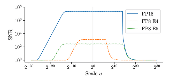
The signal-to-noise ratio (SNR) of a normal distribution quantised in FP16 and FP8, at different scales. For smaller number formats, the signal is strong over a narrower range of scales.
Unit scaling is a technique for model design that operates on the principle of ideal scaling at initialisation; that is, unit variance for activations, weights, and gradients. This is achieved by considering the change in variance introduced by each operation in the model and introducing fixed scaling factors to counteract this.
The resulting model automatically produces tensors that are well-scaled for low-precision number formats, making their use straightforward and minimising the downsides of these highly efficient representations. The overheads and additional complexity introduced are minimal, unlike alternative approaches to low-precision training.
Our method achieves breakthrough results: for the first time, we have accurately trained BERT Base and BERT Large models in FP16 and even FP8 without loss scaling. Unit scaling works out-of-the-box, with no extra sweeps or hyperparameters required for training. Unit-scaled models can then be used for inference with no additional constraints or modifications.
For practitioners who care about efficiency - and hence wish to train in FP16 and FP8 - unit scaling offers a straightforward solution. The IPU is well-suited to these use-cases, with Graphcore's current Bow IPU processor providing accelerated FP16 compute, and next-generation IPU hardware adding accelerated FP8 compute. Users can try out unit scaling for themselves through the accompanying Paperspace notebook.
Unit Scaling: a how to guide
![]()
FP16 and FP8 training require some form of scaling to keep values within range. The current approaches to this are as follows:
Reduced range is particularly challenging for the backward pass during training, often leading to underflowing gradients. To combat this, one approach is to multiply the loss by a loss scale hyperparameter to increase the size of gradients [1]. As there is no principled way to choose the loss scale ahead-of-time, this hyperparameter may need to be swept, often requiring multiple full runs.
One can avoid the need for hyperparameter sweeping by dynamically adjusting the loss scale based on run-time gradient overflows (or histograms) [2]. This can also combat shifts in tensor distributions during training. Unfortunately, automatic schemes may add overheads and complexity.
Another downside of the above methods is that they only provide a single global loss scale. One proposed solution is to re-scale values locally based on tensor statistics [3]. This is also an automatic/run-time scheme, and as such may be complex and hard to implement efficiently.
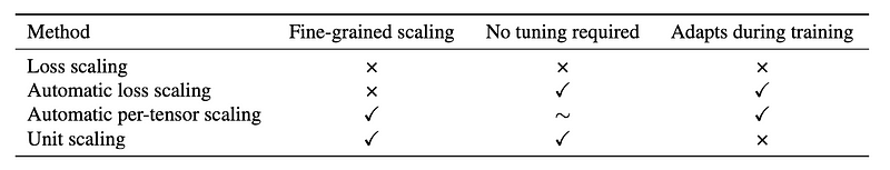
A comparison of techniques for low precision training. '∼' indicates that this method ideally requires no tuning, but in practice may introduce hyperparameters that need to be swept.
Unit scaling also introduces local scaling factors in the forward and backward pass to control the range of values. However, we choose these factors based on a theoretical understanding of how each operator affects the scale of values, rather than using run-time analysis.
By choosing the correct scaling factors, each operation approximately preserves the scale of its inputs. By applying this to all operations, this propagates the initial (unit) scale throughout the model, giving unit scaling globally.
Note that our analysis is based on the scale of values at initialisation, before training has commenced. Although scales shift during training, we find that good initial scaling gives enough headroom that re-scaling is not required (future work will investigate this direction further, evaluating the possibility of re-scaling at longer intervals as we move to larger models).
Our method is simpler than automatic scaling schemes, and the only additional overhead is that of applying the scaling factors (a scalar multiplication, that can be fused into the previous operation). For BERT Large this introduces a negligible 0.2% increase in FLOPs.
A model can be unit-scaled by applying the following recipe:
We explain these rules in more detail below.
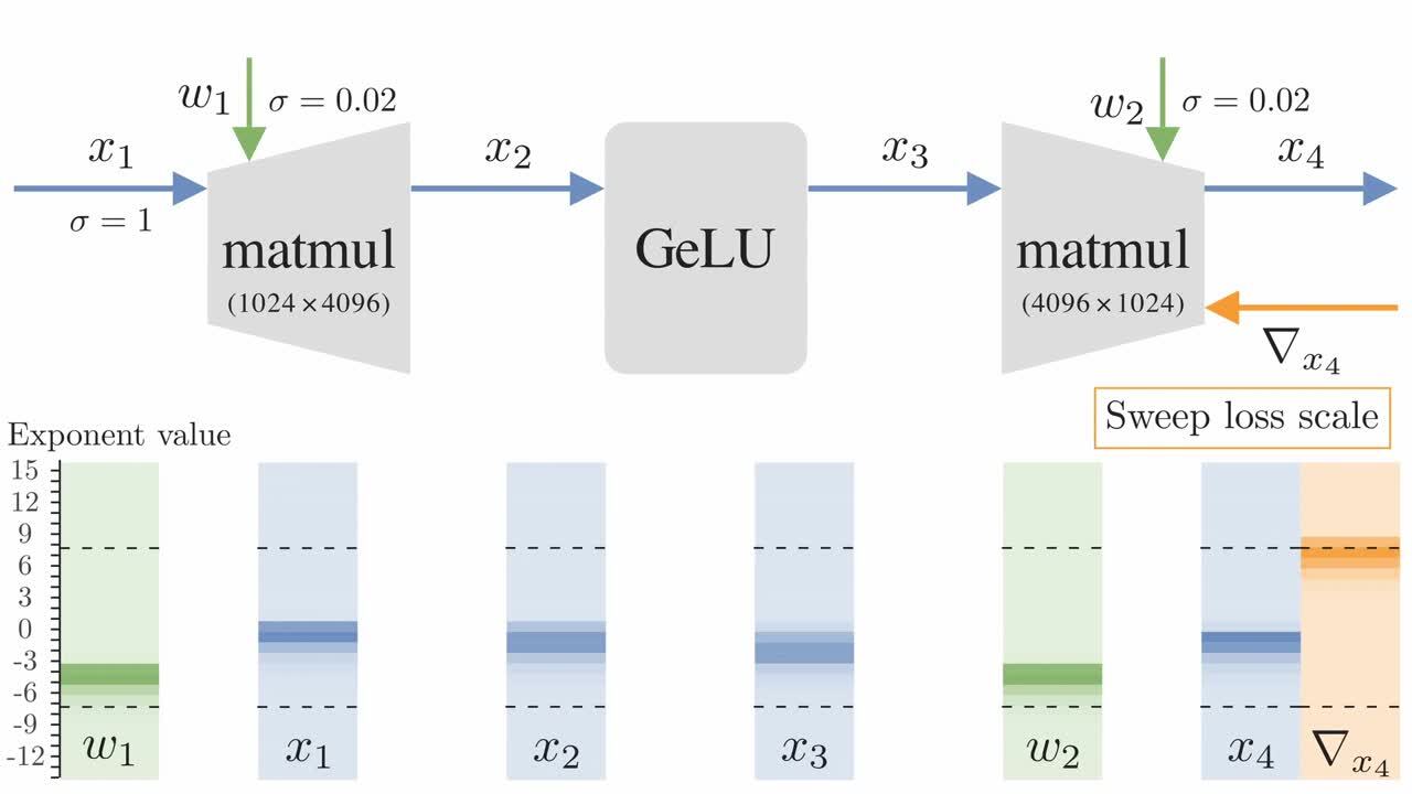
We can analyse some operations mathematically to determine how they affect the variance of their inputs.
For example, a basic matrix multiplication XW (where X is a (b × m) matrix and W is a (m × n) matrix) has an output variance of σ(X)² · σ(W)² · m. To unit-scale this operation, we must ensure σ(X)² = σ(W)² = 1 (by scaling previous operations), and then add a 1/√m multiplication to the output.
This accounts for the forward pass. The backward pass introduces two new matrix multiplications, with ideal scaling factors of 1/√n and 1/√b. Other operations can be analysed similarly, and in cases where the output variance cannot be easily analysed, empirical methods can be used to find scaling factors.
We provide a more detailed analysis in our arxiv paper, along with a compendium of common operations and their ideal scaling factors.
Directly applying these ideal scaling factors in the forward and backward passes can generate invalid gradients. To avoid this, we require that certain operations use a shared scaling factor.
Specifically, we take the forward computational graph and find all the variables that are not represented by cut-edges (edges which if removed, would split the graph into two unconnected smaller graphs). The following shows a transformer FFN layer:
.png?width=576&height=370&name=Scaling%20chart%203%20(1).png)
A visualisation of the cut-edges in an FFN layer, and the associated scaling factors.
In this case, we have cut-edges on the weight, input and output variables. The diagram also shows the generated gradient operations for the second matmul's backward pass (note: we only consider cut-edges for the forward graph).
We constrain the matmul for ∇x₃ to use the same scaling factor as in the forward pass, because x₃ is not a cut-edge. However, as w₂ is a cut-edge, it's allowed its own backward scaling factor. To choose the shared scaling factor for the constrained ops, we take the geometric mean of the ideal scaling factors calculated previously.
Though this cut-edge rule can sound complex, in practice it usually comes down to a simple procedure: giving weight gradients their own scaling factors, as well as any encoder/decoder layers in the model.
The final step of our recipe is to replace add operations with weighted adds. Unit scaling by design produces variables with equal scales, meaning if we add two tensors, both effectively have equal weight. However, in some cases, especially residual connections, we might require an imbalanced weighting to attain good performance.
To account for this, we replace add operations with a weighted (and unit-scaled) equivalent. For residual connections, we use this to derive the following recommended schemes:
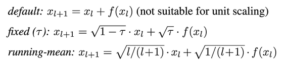
Residual connection schemes for unit scaling.
The following code shows an implementation of a unit-scaled FFN layer in PyTorch. We provide further example implementations in our codebase and demo notebook.
We first define some scaling primitives, which allow us to create scaled versions of basic ops, such as scaled_projection:
This then allows us to create full scaled layers. Here we demonstrate a standard FFN and its unit-scaled equivalent:
Our experimental results demonstrate that unit scaling is effective across a wide range of models, and works out-of-the-box, with no additional hyperparameter-tuning needed.
Our first set of experiments validates the broad applicability of unit scaling across different model architectures. We trained a large variety of smaller character-level language models with and without unit scaling, in both FP32 and FP16, and compared the results. These configurations amount to a 2092-run sweep:.png?width=489&height=495&name=Scatter%20charts%20(1).png)
Character language modelling, showing validation bits-per-character over a wide range of models. Each point represents one combination of: {Conv, RNN, Attention}, {Pre, Post, No norm}, {Fixed, Running-mean residual}, {SGD, Adam}, {2, 8 Layers}. Each point is the best final value over a learning rate sweep.
Our results demonstrate the following: first, that some form of scaling (loss or unit) is required when using FP16. This is due to gradient underflow, since loss scaling with a factor of 2048 resolves the issue. Second, that unit scaling, despite changing the training behaviour of the model beyond just numerics, matches or even slightly improves upon baseline performance in almost all cases. Finally, that no tuning is necessary when switching unit scaling from FP32 to FP16.
Our second set of experiments validates the effectiveness of unit scaling on a larger and more realistic production-grade model, BERT [4]. We apply adjustments to our unit scaled model to align it with a standard BERT implementation, and then train it on text from English Wikipedia articles.
Our results on SQuAD v1.0 and SQuAD v2.0 evaluation tasks are as follows:
.png?width=575&height=199&name=Another%20table%20(1).png)
We pretrain 3 models for every model-method-format combination, then fine-tune 5 SQuAD v1.1 and 5 v2.0 runs for each. Values shown represent the mean across the 15 runs, with ± indicating standard deviation across the mean scores of the 3 sub-groups.† from Devlin et al. (2019). ‡ from Noune et al. (2022).
Unit scaling is able to attain the same performance as the standard (baseline) model, and whereas the baseline requires sweeping a loss scale, unit scaling works in all cases out-of-the-box. The baseline and unit-scaled models aren't exactly equivalent, but deviations in their downstream performance are minor (unit-scaled BERT Base is slightly below the baseline, and BERT Large is slightly above).
Our FP8 implementation is based on the formats recently proposed for standardisation by Graphcore, AMD and Qualcomm. Graphcore research previously demonstrated the training of loss-scaled BERT in FP8 with no degradation [5], and we now show that the same can be achieved with unit scaling.
No additional techniques are required to make FP8 work over FP16. We simply quantise our matmul inputs into FP8 and are able to train accurately (with weight and activations in the FP8 E4 variant, and gradients in E5). These results represent the first time BERT Base or BERT Large have been trained in either FP16 or FP8 without requiring loss scaling.
As the adoption of hardware with FP8 support grows within the AI community, so too will the importance of effective, straightforward, and principled approaches to model scaling. Unit scaling satisfies all of these criteria. It's also applicable across a broad range of models and optimisers, with minimal computational overhead.
The next generation of large models will likely make extensive use of low-precision formats, and hence may require a unit-scaling-like approach. We hope that our method can be of use for these applications, and also lay a strong foundation for future scaling research. The efficiency benefits of low-precision training are substantial, and unit scaling shows they don't have to come at a cost.
Read the paper | Code | PyTorch demo notebook
[1] P. Micikevicius et al., Mixed precision training (2018). 6th International Conference on Learning Representations
[2] O. Kuchaiev et al., Mixed-precision training for nlp and speech recognition with openseq2seq (2018), arXiv preprint arXiv:1805.10387
[3] P. Micikevicius et al., FP8 formats for deep learning (2022). arXiv preprint arXiv:2209.05433
[4] J. Devlin et al., BERT: Pre-training of deep bidirectional transformers for language understanding (2019). NAACL-HLT
[5] B. Noune et al., 8-bit numerical formats for deep neural networks (2019). arXiv preprint arXiv:2206.02915
Share: