Oct 04, 2022
Oct 04, 2022
We're Hiring
Join us and build the next generation AI stack - including silicon, hardware and software - the worldwide standard for AI compute
Join our teamIn this blog post, we will introduce an original technique developed by Graphcore to reliably and easily improve stability when training large models in mixed precision. Its origin lies in our unique experiences developing applications for IPUs, and it has now been integrated into our Poplar SDK for ease of use. Our ongoing aim at Graphcore is to make the process of developing models and experimenting on IPUs as easy as possible for users with a range of different needs and levels of familiarity—from ML researchers to data scientists, MLOps engineers, cloud applications developers, and beyond.
We will start by explaining why loss scaling plays a vital role in mixed-precision training of large models, particularly given the trends driving advancements in machine learning. We will demonstrate how all loss scaling methods to date (manual and automatic) have suffered from inefficiencies or are prone to failing. We will then show how the Graphcore ALS algorithm offers a much-needed combination of efficiency, ease of use, and remarkable stability.
Many breakthroughs in machine learning have been enabled by a continuing increase in size and complexity of model architectures. Lower precision numerical formats are a critical tool in overcoming the computational challenges that accompany the trend towards larger models, yielding several benefits: lower memory footprint, greater bandwidth and throughput, and more energy-efficient training thanks to reduced power consumption. However, these benefits come at the cost of introducing numerical instabilities during training and reducing the statistical performance of some models. For current large deep learning models, practitioners usually employ a mixture of IEEE 32-bit and 16-bit floating point representations during training — this is called mixed-precision training. In this blogpost we explain why loss scaling is needed to make mixed-precision training converge well, and how we can automatically adjust it during training from observing gradient histograms.
Reducing the precision from IEEE float-32 to IEEE float-16 narrows the dynamic range of the activations, weights, and gradients. As models get larger and deeper, gradients become smaller and it is crucial to ensure that their signal is not lost due to underflow in float-16. Similarly, models can tolerate a certain level of overflow, but in excess it can lead to instabilities and sudden failures. All in all, both underflow and overflow hamper training convergence. An alternative to float-16 precision is bfloat-16, which was introduced by Google and maintains the dynamic range of float-32 by reducing the mantissa bits. bfloat-16 reduces the risk of underflow or overflow of gradients and no loss scaling is needed, but this comes at the cost of potentially hampering statistical convergence. This was shown in Google’s Gopher training paper, where the authors found that using bfloat-16 degrades performance by comparison with float-32, even when complementing it with techniques such as stochastic rounding.
Loss scaling aims to shift the gradient distribution across the dynamic range, so that underflow and overflow are prevented (as much as possible) in float-16. As the name suggests, gradients are scaled by multiplying the loss function by a constant factor. Consequently, gradients obtained through back-propagation are also scaled by that constant. This scaling has to be taken into account during the weight update, since otherwise the training would be affected by the loss scaling value. The image below summarizes the loss scaling method for the SGD optimiser.
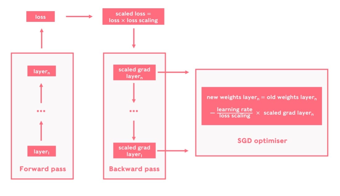
Loss scaling applied with the SGD optimiser
Choosing the loss scaling factor manually is a time- and resource-consuming endeavour. Moreover, due to the dynamic evolution of gradient distribution a static value for loss scaling may not remain optimal throughout training. The Graphcore ALS solution makes training in float-16 easier to use and more stable by addressing these concerns.
Large models are known for their instabilities during training, which may be due to numerical issues or even hardware failures. However, this practical topic is usually not emphasized in scientific publications: most interest is given to validation scores of the model, with rather less attention paid to the challenges involved in multiple attempts to train large models in a stable fashion.
Tuning loss scaling in mixed-precision training is a prime example of such a challenge. Tuning can be done manually or via a dynamic or automatic procedure which chooses a loss scaling value per step or interval of steps according to a certain criterion. There are several proposed approobserveaches for designing automatic procedures in the literature. One approach, based on the occurrence of NaN values in computations, was recently employed by Meta’s engineers in their recent OPT-175B model. However, a quick review of mentions of loss scaling in Meta’s training logbook reveals that, for many attempts, training stably was impossible due to loss scaling exploding unexpectedly, which led to sudden instability in the loss function and lack of convergence. This is clearly an unexpected behaviour of their dynamic loss scaling procedure, whose aim is really to stabilize training.
At Graphcore we have refined such loss scaling procedures thanks to our experience understanding the failure modes that large models typically display. This has allowed us to strengthen the training stability of large models by developing efficient in-house tools in our Poplar SDK. Before getting into the details of the Graphcore ALS algorithm, let's first see how BERT Large can fail due to a wrong choice of static loss scaling.
We pretrain phase 1 of BERT Large on an IPU-POD64 following the hyperparameters in the paper Large Batch Optimization for Deep Learning: Training BERT in 76 minutes, where the LAMB optimizer is introduced. We use float-16 representations for all weights, activations, and gradients. Only the first and second moments of the LAMB optimizer are set to float-32. You can find our open-source implementation based on Hugging Face transformers and details about the dataset in our GitHub repository.
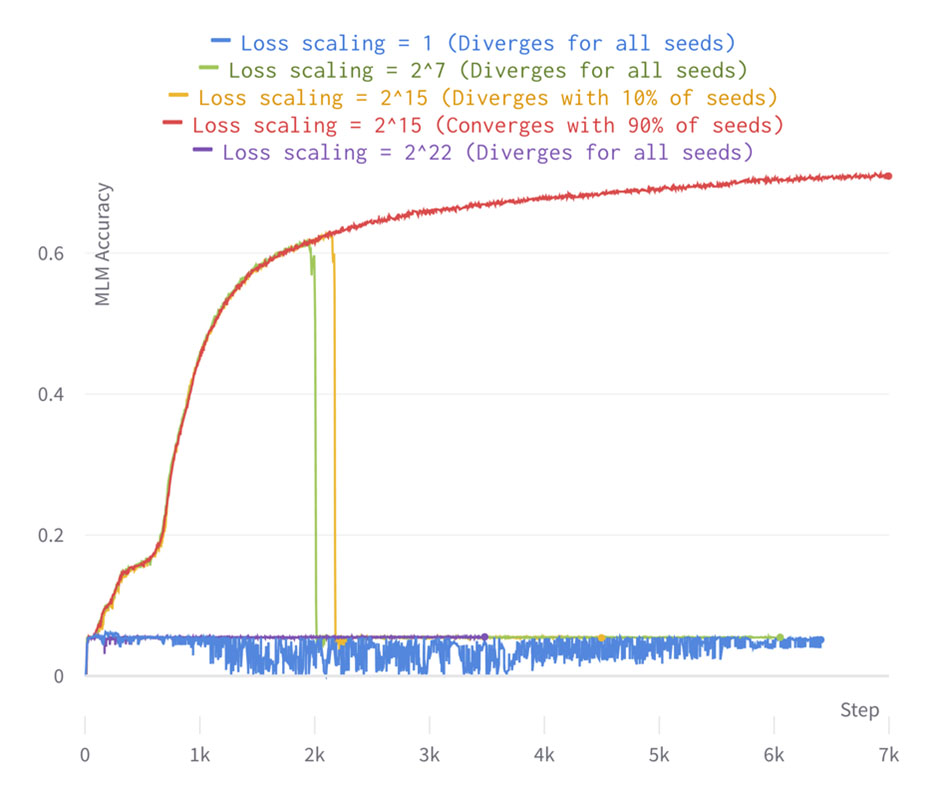
The image below depicts the training evolution of BERT Large with four constant different values of the loss scaling. For the loss scaling values of 1, 27and 222, training diverges no matter the seed selected. For values between 27 and 222, the run converges depending on the seed, with a lower or higher probability of converging. In particular, setting loss scaling at 215 leads to the highest convergence rate of 90% (i.e., only 10% of the seeds end up diverging during training). For simplicity we only plot one of the diverging and converging seeds, but the experiments have been repeated for many other seeds. This means that, when using static loss scaling, there may be a risk of diverging no matter the loss scaling value selected. However, choosing the right loss scaling value is crucial to ensure that the diverging rate is as low as possible.
We observe that the run with loss scaling equal or lower to 1, and higher than or equal to 222, always fails quite early. This is due to a significant gradient underflow/overflow in float-16 and the run is unable to progress beyond the beginning of training. The run with loss scaling equal to 27 progresses adequately until 2k training steps, which is when the learning rate scheduler reaches its peak (as shown below) and the run becomes more unstable. At this point the run catastrophically fails within only a few training steps. This is also around when the runs with loss scaling 215 fail for 10% of seeds. Sudden failures such as these are quite characteristic of large models, and there's some debate in the community about how they are caused, whether gradient underflow or overflow is involved, and which gradients with respect to weights or activations are responsible for them.
MLM accuracy of BERT large phase 1 pretraining for various loss scaling choices
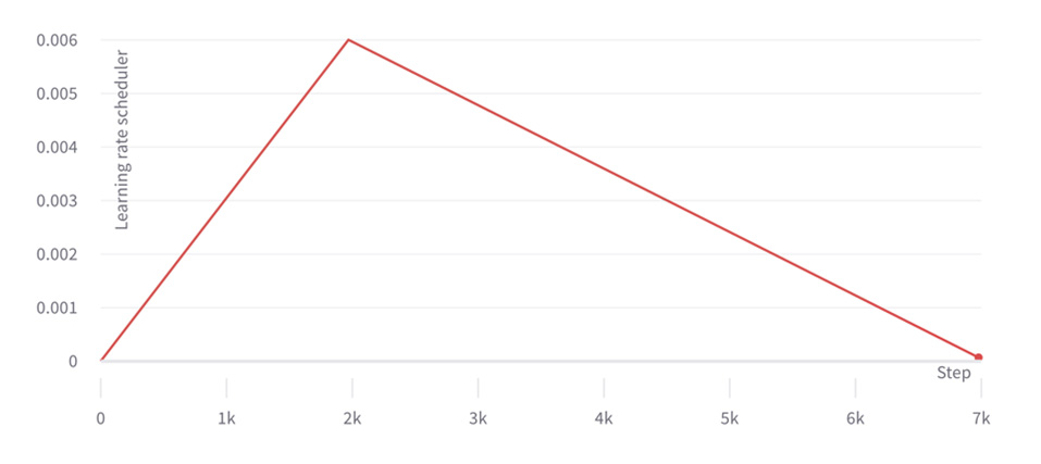
Learning rate scheduler for BERT large phase 1 pretraining
In any case, it is clear that finding an appropriate loss scaling is paramount for training stability: all of the displayed BERT runs share identical hyperparameters but differ in terms of loss scaling factor and seed. Optimising loss scaling can lead to convergence for most of the seeds.
We should also note that finding the appropriate loss scaling values can be pretty expensive – consuming hours or even days of compute time, depending on the system used.. If this needs to be repeated for several loss scaling sweeps, the computational resources consumed can escalate significantly.
This problem is solved by the Graphcore ALS algorithm as presented in the next section, which allows us to reach 100% convergence rate for the BERT training configuration shown above.
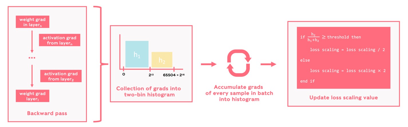
The Graphcore ALS approach is based on observing the gradients with respect to both weights and activations. These observations are used to generate histograms that inform the adjustment of the loss scaling factor, with the aim of preventing excessive underflow or overflow in gradient distribution. This approach differs from other strategies, which generally involve tuning the loss scaling factor based on the occurrence of NaN/Inf values in the computations when an overflow event takes place. We believe that observing the gradients is a more informed strategy since it can balance the amount of overflow and underflow.
We aggregate the gradients into histograms with just two bins—h1 and h2—covering the full dynamic range of float-16 (i.e., from 0 to 65504). Whenever an overflow event takes place, the value remains clipped at the maximum numerical representation, which in float-16 corresponds to 65504. Due to this clipping, we may miss overflow events taking place during intermediate operations if we only focus on the final values. To also take these intermediate overflows into account, we set the bin edge between both bins to be close to overflow but leaving some margin, and in practice bin edges such as 213 have resulted in stable runs. We compute the ratio between the two bins with each weight update, and depending on a threshold value taken as 10-7 we either double or half the loss scaling value. The diagram below visually describes our ALS algorithm.
ALS algorithm diagram
The logic behind the algorithm is simple: the loss scaling keeps doubling to prevent underflow. The loss scaling is halved to avoid excessive overflow only when the upper bin counts reach a certain proportion compared to the sum of both bins.
The algorithm can be adjusted to reduce its computational overhead: it is possible to introduce a period, which makes sense since the gradient distributions changes slowly for most models, meaning that the loss scaling factor does not need to be adjusted after every training step.
Another possible modification concerns the gradients to track: picking only the ones from certain layers/operations, weight gradients, activation gradients, etc., instead of all gradients, but this may result in model-dependent ALS schemes that may not be generally applicable. For simplicity, in this blogpost we set the period as 1 and track all gradients.
To test the ease of use and robustness of the Graphcore ALS algorithm, we apply it to pretraining two of the most popular deep learning models in recent years: BERT large (BERT) for language and EfficientNet-B4 for vision.
BERT (as in the static loss scaling example earlier) is trained according to the paper Large Batch Optimization for Deep Learning: Training BERT in 76 minutes, whereas Efficient-B4 base follows the reference paper EfficientNet: Rethinking Model Scaling for Convolutional Neural Networks but with the algorithmic improvements suggested in Making EfficientNet More Efficient: Exploring Batch-Independent Normalization, Group Convolutions and Reduced Resolution Training.
In both models we keep all weights and gradients in float-16 apart from the optimizer state, which is in float-32. Partial operations are carried out in float-16 too. The optimiser is LAMB for BERT and RMSProp for EfficientNet, and the learning rate follows a warmup initial stage until reaching the maximum (at 2k training steps for BERT phase 1, 275 steps for BERT phase 2, and 4 epochs for EfficientNet), followed by a linear learning rate decay for BERT (resp. exponential for EfficientNet) until the end of the training.
Graphcore’s open-source implementation of BERT, based on HuggingFace Transformers, can be found in our GitHub repository together with details about the Wikipedia dataset. Similarly, our in-house open-source implementation of EfficientNet, together with details about the ImageNet dataset, are located in our GitHub repository.
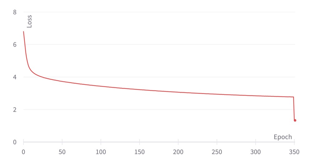
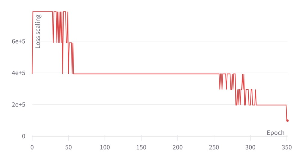
The training plots for BERT are shown in the graphs directly below. Training BERT comprises two phases: the first uses sequence length 128, and the second 512. This is mainly for efficiency: attention is quadratic in sequence length; training with a shorter sequence length is cheaper, but training with a longer sequence length is needed to learn the positional embeddings and long-range dependencies.
We observe that at the end of phase 2, the loss function reaches a value of 1.24. This is a SOTA score that leads us to achieve an exact match of 84.38 and F1 of 90.92 when fine-tuning in SQuAD (the reference from the BERT paper is 84.1 and 90.9 respectively). Concerning the loss scaling plots, we initially set the loss scaling value to 1, but then it is adjusted after every training step, leading to a zig-zagging profile that tends to oscillate around 215=32,768 for phase 1 and 214=16384 for phase 2. The zig-zag is produced after every training step since the loss scaling update period is set to 1, but one could use less frequent updates too.
Interestingly, we see that for phase 1 the loss scaling value remains oscillating and somehow constant throughout training, except during some steps between 1k and 2k—this is where the learning rate reached its highest value in the previous pretraining example using static loss scaling. The Graphcore ALS algorithm reacts to a change in the gradient distribution, which could be due to a larger variance in the distribution or larger overall values. In any case, the algorithm decreases the loss scaling value to prevent excessive overflow.
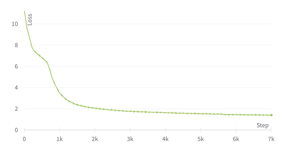
Loss evolution for BERT large pretraining phase 1 with ALS
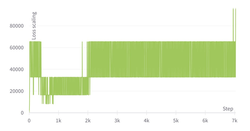
Loss scaling evolution for BERT large pretraining phase 1 with ALS
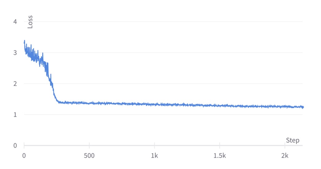
Loss evolution for BERT large pretraining phase 2 with ALS
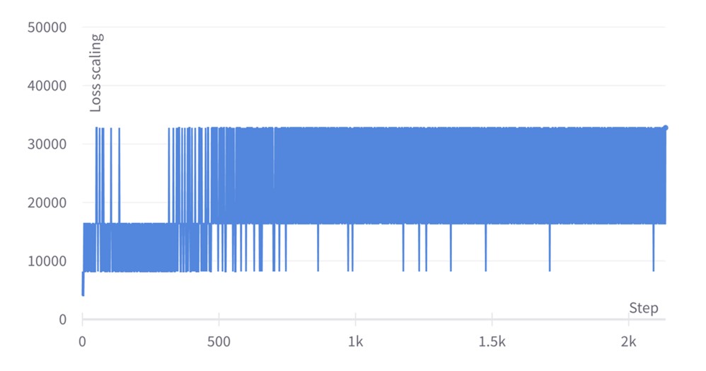
Loss scaling evolution for BERT large pretraining phase 2 with ALS
The training plots for EfficientNet are shown in the graphs below. Instead of plotting at each training step, we just plot the final value of the loss and loss scaling per epoch. The loss function smoothly decreases during training, reaching a final validation accuracy of 82.33 which agrees with the reference value of 82.3 in Making EfficientNet More Efficient: Exploring Batch-Independent Normalization, Group Convolutions and Reduced Resolution Training.
The final drop in loss results from computing the last checkpoint as an exponential moving average of all the previous checkpoints. With regards to the loss scaling evolution, the constant-wise profile is due to just plotting once for every epoch; in reality, the loss scaling is still being updated after every weight update, in a similar fashion as for BERT above. There's also some variation in the optimal loss scaling value throughout training.
Loss evolution for EfficientNet-B4 pretraining with ALS
Loss scaling evolution for EfficientNet-B4 pretraining with ALS
There are sporadic spikes in the loss scaling profiles for both the BERT and EfficientNet, demonstrating that the Graphcore ALS algorithm is able to detect local events that could potentially lead to training divergence, such as problematic data batches. In contrast to other automatic loss scaling schemes, which avoid updating the weights whenever a NaN even takes place, our scheme can continue training regardless since gradients are clipped to the maximum float-16 value and the loss scaling is adjusted accordingly.
While loss scaling is essential to shift gradients appropriately in the dynamic range and prevent underflow, it may not be enough depending on the model and configuration. To enhance stability, at Graphcore we complement loss scaling with stochastic rounding, running mean for accumulations and float-32 precision for certain elements such as the optimiser state moments.
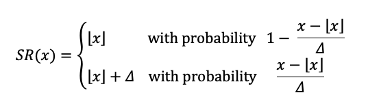
Stochastic rounding, natively supported by the IPU, can be used with mixed precision training to help alleviate precision loss when using float-16 partials (in 16.16 AMPs) or to enable training without a float-32 copy of the master weights. With stochastic rounding, the decision about which output to produce is non-deterministic: for instance, when stochastically rounding 1.2, 20% of the time the result is 2 and 80% is 1. This differs from the nearest-value rounding, where the decision is deterministic and rounding 1.2 always results in 1. Mathematically, for an input x with quantization step Δ, the stochastic rounding formula is:
 Stochastic rounding has the benefit of producing an unbiased quantisation (where $\mathbb{E}\{ SR (x)\}=x$) despite adding a level of tolerable error. This means that, over many such additions, the added quantisation noise has zero mean, and the count of injected carries approximates what would have been propagated by accumulation at higher precision.
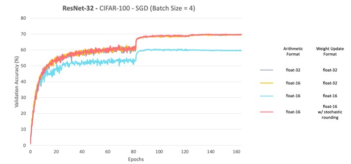
As an example, let’s look at the impact of stochastic rounding in ResNet32 with CIFAR-100, SGD and a batch size of 4. The graph below compares the validation accuracy achieved for different combinations of float-32 and float-16 precisions for the arithmetic and weight update format. Enabling stochastic rounding prevents the degradation of validation accuracy when float-16 is employed in both arithmetic and weight update format.
The second strategy to enhance stability involves performing accumulation operations with a running mean. Neural network architectures typically employ large batch sizes per weight update to save communication costs per weight update. Unfortunately, such batch sizes usually don’t fit in memory, meaning that the gradients of all the batch samples cannot be computed in one go. To surmount this while keeping batch sizes large, there are various strategies to parallelise/serialise gradient computation and save memory — here we highlighted two of them:
For both data parallelism and gradient accumulation, there’s an accumulation operation that needs to be performed with the aim of computing the mean of the gradients. If the mean is computed firstly by adding all gradients and secondly dividing over the total number of gradients, there’s a risk of overflow in float-16.
Consequently, we have implemented a running mean accumulation that ensures that the accumulated gradient is no larger than the magnitude of the largest micro-batch gradient for both data parallelism and gradient accumulation.
In particular, given gradients $g_{1},\dots, g_{N}$ the mean of the first $k$ gradients is calculated iteratively by computing
\[M_k = \frac{k-1}{k} M_{k-1} + \frac{1}{k} g_k\]
with $M_0=0$. Running mean is actually necessary to decouple the loss-scaling tuning and the accumulation scale, since with it both the gradients and their accumulation have the same order of magnitude.
While loss scaling is an essential tool for mixed-precision training, setting the scaling factor manually is a time and resource-intensive process; meanwhile, automatic approaches are prone to failure.
In this blog post, we have introduced Graphcore’s own ALS algorithm, which uses a unique histogram-based loss scaling approach to prevent underflow and overflow, ensuring that models converge. We have demonstrated how our ALS algorithm yields 100% convergent pretraining runs on BERT and EfficientNet, with loss scaling being adjusted after every training step.
Graphcore ALS is accelerator-agnostic and can be applied beyond IPUs. It has been integrated into Graphcore’s Poplar SDK on an experimental basis for a while, and with the release of Poplar SDK 3.0 moves to “in preview.”
Graphcore ALS is also fully enabled in many of our PyTorch applications; currently supported applications include:
Additionally, it is quite simple to enable Graphcore ALS for almost any PyTorch model with a few additional lines of code when creating the model:
opts.Training.setAutomaticLossScaling(True)
poptorch_model = poptorch.trainingModel(model, opts, optimizer=optimizer)
This ensures that Graphcore ALS is enabled and passed when instantiating the model you are training.
We should point out, however, that while Graphcore ALS works perfectly in most cases, it is not guaranteed to work on all models.
Our ongoing aim at Graphcore is to make the process of developing models and experimenting on IPUs as easy as possible for users with a range of different needs and levels of familiarity—from ML researchers to data scientists, MLOps engineers, cloud applications developers, and beyond.
Share: