Aug 31, 2022
Aug 31, 2022
We're Hiring
Join us and build the next generation AI stack - including silicon, hardware and software - the worldwide standard for AI compute
Join our teamFraser King is a Ph.D. student at the University of Waterloo (Ontario, Canada). A version of this post first appeared in Towards Data Science. Graphcore's support in drafting this post has been limited to providing technical support and guidance related to IPU systems and technology.
The application of machine learning (ML) in the Geosciences is not a new idea. Early examples of k-means clustering, Markov chains and decision trees have been actively used in several geographical contexts since the mid-1960’s (Preston et al., 1964; Krumbein et al., 1969; Newendorp, 1976).
However, advancements in cloud computing resources from companies like Graphcore, Amazon and Google, combined with the ease-of-access to powerful ML libraries (e.g. Tensorflow, Keras, PyTorch) and flourishing developer communities, has allowed this emerging field to explode in popularity in recent years (Dramsch, 2020).
Now, ML models are not only regularly used in the Geosciences for operational forecasting (Ashouri et al., 2021), but for statistical inference as well; without the traditional uncertainties associated with physical model simulations of natural processes (King et al., 2022).
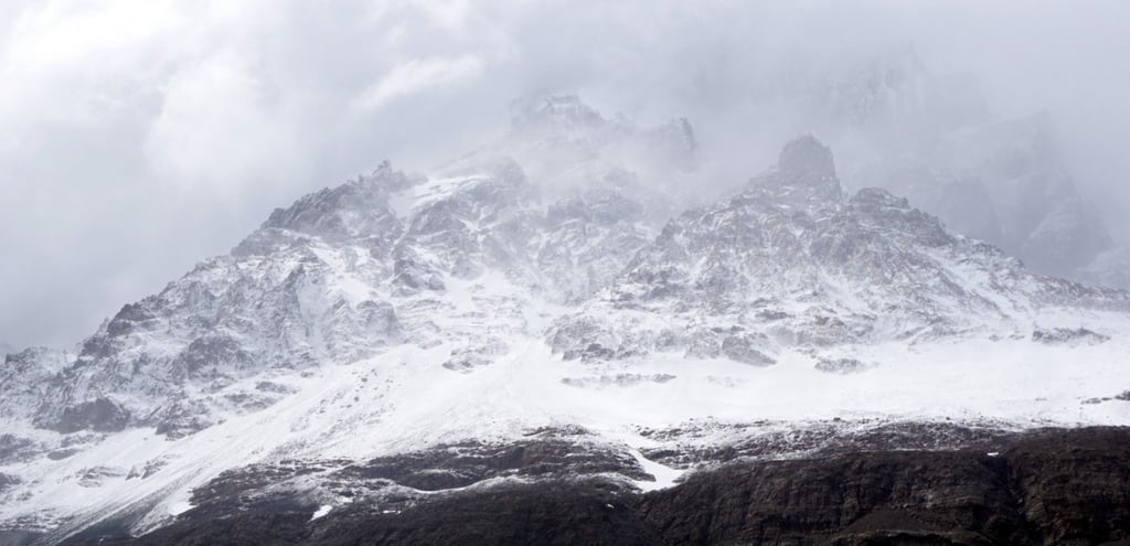
Snowfall is an integral component of the global water and energy cycle with significant impacts to regional freshwater availability (Musselman et al., 2021; Gray and Landine, 2011). In fact, over 2 billion people (a sixth of the global population) rely on snowmelt-derived fresh water for human consumption and agricultural purposes each year (Sturm et al., 2017). As global mean temperatures continue to rise, snowfall frequency and intensity is also expected to change, leading to new water resource management challenges worldwide (IPCC, 2019).
However, traditional snowfall models have large uncertainties in their estimates and therefore new algorithms should be investigated to advance our understanding of shifting global snowfall patterns.
 So, let’s explore how ML is being used to advance the field of snowfall prediction, and where these techniques may lead in the future.
Illustrated at the top of this post is DeepPrecip. Or more accurately, a render of DeepPrecip’s compute graph that forms the basis of the model’s decision making process.
DeepPrecip is a deep convolutional neural network (CNN) developed at the University of Waterloo comprised of 4 million trainable model parameters! Our goal with this model is to evaluate how well we can use ground radar data inputs to predict surface precipitation quantities under varying regional climates (King et al., 2022–2). This type of model is known as a precipitation “retrieval” as the inputs to this model are atmospheric radar observations (i.e. power backscattered from falling hydrometeors) and it outputs predictions about surface rain and snow.
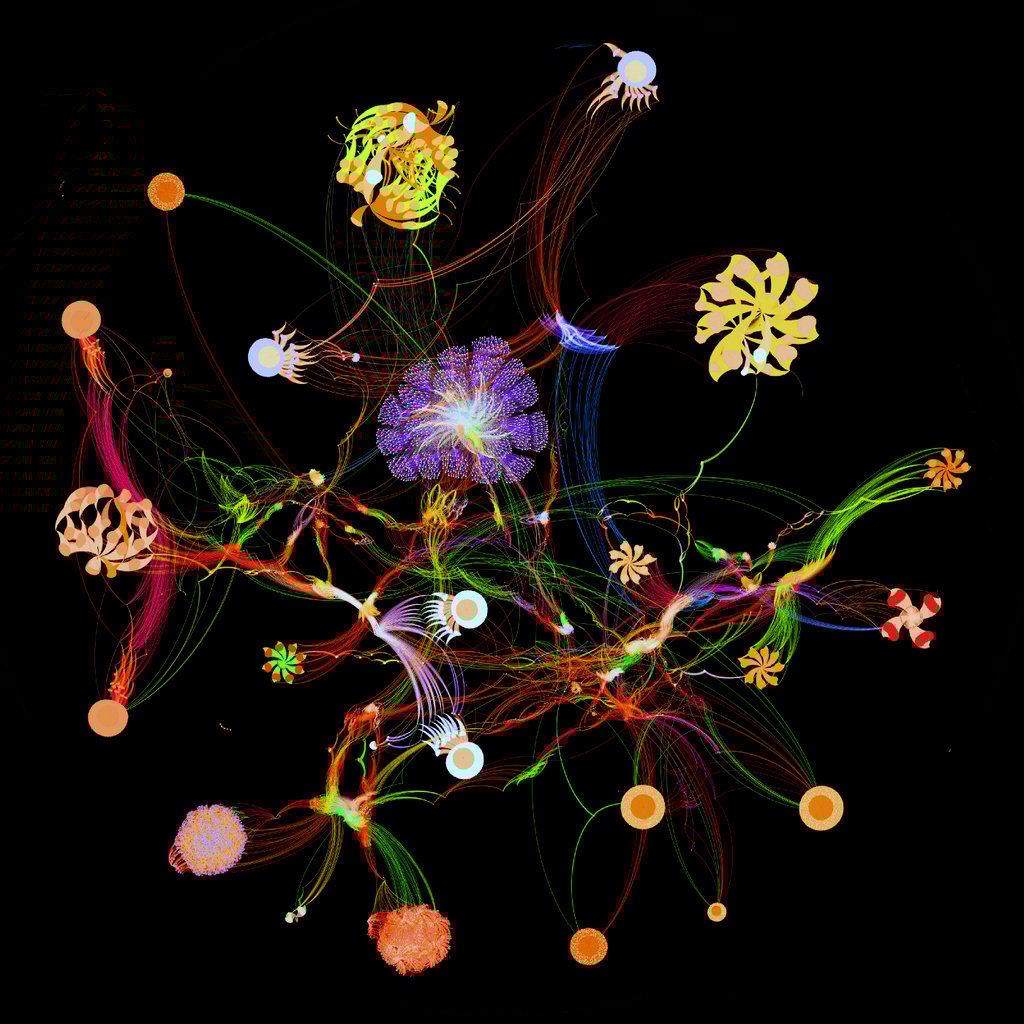
DeepPrecip network compute graph rendering — Image by Graphcore and Author
But how can atmospheric radar backscatter intensity be used to infer surface precipitation quantities?
Well, we must find a way to extract very specific information about precipitation from only partially-related atmospheric variables of interest (which in this case is radar backscatter intensity). This can be accomplished in two ways:
1. Through a physically-based model which simulates the physical processes occurring in the atmosphere resulting in the formation of ice crystals and eventually falling snow.
2. Empirical statistical processes (e.g. ML models) which can find patterns between disparate variables that display some sensitivity between one another through a forward model.
While both techniques have their own sets of advantages and disadvantages which we could spend the entire blog post discussing, we will focus on the second method in this work. But first, what is a forward model? A classic illustration is provided in Stephens, 1994:
“Suppose that you desire a description of a dragon but you observe only the footprints that the dragon makes in the sand. Now, if you already know the dragon, you can pretty easily describe the tracks it might make in the sand; i.e., you can develop a forward model. But if you observe only the tracks in the sand, it will be much more difficult to describe the dragon in any detail. You will likely be able to tell that it was a dragon and not a deer, but there will be aspects that you will be unable to characterize: the dragon’s color, if it has wings, etc. A retrieval can combine the observations (large footprints) with prior information (most dragons have wings and the ones making large footprints are green) to get the most likely state (it was a green dragon with wings).”

Dragon footprint in sand — Photo by Vishy Patel on Getty Images
We can use this idea to relate the information in the vertical radar profile to surface snowfall quantities! Since there is a physical structure to the radar data inputs (profiles reach from the surface up to about 3 km), multiple convolutional layers are employed by DeepPrecip to extract features between different portions of likely hydrometeor activity. This information helps our model understand different storm event types and structures which improves the accuracy of the intensity of the precipitation rate estimate in the fully connected feedforward regression component of the network.
More formally, the model architecture for DeepPrecip is shown below. Can you match different model architecture layers from this image to the earlier shown compute graph?
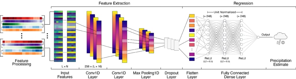
DeepPrecip model architecture diagram — Image by Author
In order to develop a robust model, we first need to gather a representative training dataset of radar data and collocated in situ precipitation measurement observations. Note that this is a supervised learning problem and therefore reference data is required.
As is always a challenge with problems in the Geosciences, care must be taken during the data selection phase to choose a representative sample. Each site must also be equipped with similar instruments calibrated in the same manner. In this work, we settled on 9 sites from across the northern hemisphere with 8 years of data collected from micro rain radar (MRR) systems and Pluvio2 gauges. Examples of these instruments are shown below.
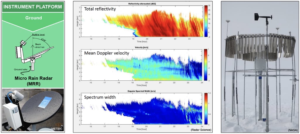
MRR and Pluvio2 instruments and example reflectivity profiles — Image by Author
Due to the large size of the training dataset we curated (millions of training samples) coupled with the general complexity of the model architecture, hyperparameter optimization became a bottleneck for us early on in the development process. After experimenting with a variety of different cloud computing options, the systems at Graphcore stood out as an excellent option for substantially improving our training times.
The key to this training speedup at Graphcore were the use of their specialized Intelligence Processing Units (IPUs). The IPU is a completely new kind of massively parallel processor to accelerate machine intelligence. The compute and memory architecture are designed for AI scale-out. Note the differences between IPUs and traditional processors below:
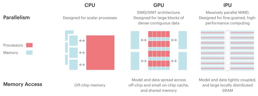
Differences between IPU architecture and other processor designs — Image by Graphcore
The hardware is developed together with the software, delivering a platform that is easy to use and excels at real-world applications. Using a Graphcore MK2 Classic IPU-POD4 (note that a second-generation IPU is now available), we were able to speed up training times by a factor of 6 for DeepPrecip over other state-of-the-art systems (e.g. Tesla V100s). If you’d like to test IPU systems for your project, check out their cloud platform.
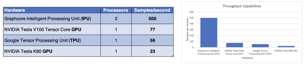
Hardware throughput comparisons for DeepPrecip training — Image by Author
With the hardware selected, we then needed to select an optimization paradigm. In order to identify the optimal hyperparameter values for DeepPrecip, we decided to use a form of adaptive optimization known as hyperband optimization. This method is a variation of Bayesian optimization (i.e. an adaptive search) which focuses on speeding up the random search process using adaptive resource allocation and early-stopping (Li et al., 2018). This allows us to test a vast hyperparameter space and quickly hone in on good values for our model parameters.
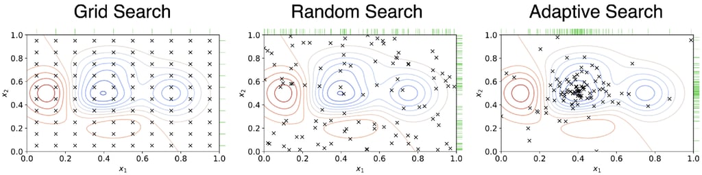
Different hyperparameter optimization techniques — Image by Talaat et al., 2022
Running a hyperband optimization of 14 different parameters for DeepPrecip with 68 different total value options (i.e. trillions of possible combinations) using a single IPU took approximately two weeks. Mean square error (MSE) metrics (below) show how this process was intelligently selecting better combinations of hyperparameters, while also slowly increasing the number of epochs each cycle.
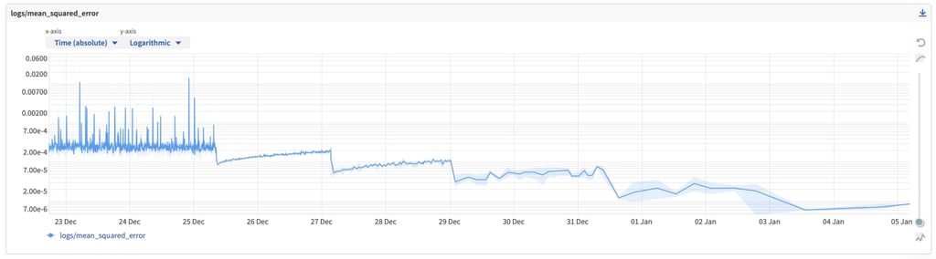
Improvements in model skill from successive hyperband optimization steps — Image by Author
A high-dimensional visualization of these parameter relationships can be rendered using a parallel coordinate plot for each iteration (or index) of the hyperband optimization process (shown below). This allows us to find a balance between the complexity of the model architecture and performance to produce a model that is both efficient and skillful. For additional details on this process along with the final hyperparameter values, please see King et al., 2022–2.
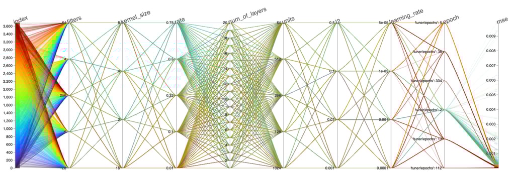
Parallel coordinate plot of each hyperparameter combination — Image by Author
While the time invested in gathering, preprocessing and properly sampling the data combined with the 2-week hyperparameterization process may seem like overkill, it is extremely important to perform these steps properly, as it significantly reduces the chances of overfitting issues down the road.
With a fully trained model on our hands, we were able to assess its general performance against other ML models and traditional empirical relationships.
In general, DeepPrecip was found to outperform other traditional retrieval methods with 40% lower MSE values and a 40% improvement in R². We also note that DeepPrecip appears much more capable of correctly estimating the peaks and troughs of high intensity precipitation compared to the other models tested. Using a cross-validation approach, we found that DeepPrecip demonstrates robustness with an improved ability to accurately predict precipitation quantities at sites with regional climates previously unseen by the model.
This last point about robustness is key. One of the major limitations of previous empirical methods was the fact that each model was bespoke for the climate in which it was derived (Wood et al., 2014). So while a model might work well in the northern USA, it might not perform well in Sweden, or in Korea, for instance.
A substantial benefit of an ML-based approach is that it can be trained on data from a variety of different locations in a manner which is unconstrained by physical assumptions of particle microphysics. We have found from this project that an ML-based solution to surface snowfall displays both low error and high generalizability and there is good reason to believe that a global ML retrieval algorithm could help enhance current satellite-based products that provide estimates of snowfall around the world.
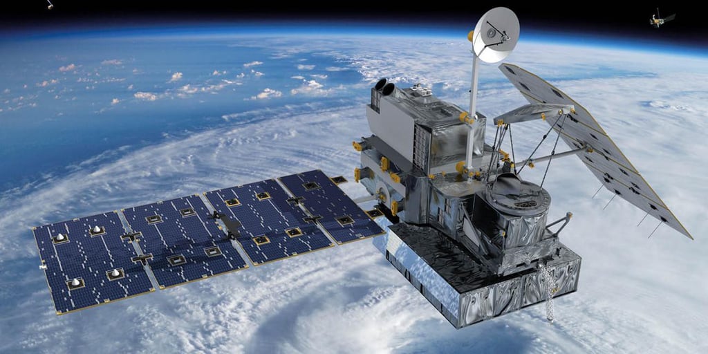
Global Precipitation Measurement (GPM) Core satellite above a hurricane — Image by NASA
The goal at the start of this project was to not only develop an operational model, but to interpret said model to identify regions within the vertical radar profile that appear as the most significant contributors to high model skill.
DL models have commonly been considered “black box” algorithms, where some input is fed into the model and some output comes out; without much of an idea of what is happening in between these two stages. Some ML models like random forests provide a feature importance ranking based on the manner in which decisions are being made by each decision tree, but how can we extract something similar for a DL model like DeepPrecip?
Enter, Shapley values.
Introduced by (and named after) Lloyd Shapley in 1951, a Shapley value is a solution concept in cooperative game theory. This value represents the contribution to some shared goal in a game from an individual participant. With multiple players, it allows us to measure the marginal contribution of each player to the end result. For instance, if multiple people go out to eat for dinner and each person orders a different main course, if we then decide to split the dinner bill, the percentage each person pays can be split based on the Shapley value.
An visual diagram describing how local explanations from a large sample of observations can provide insights on global model behaviour using Shapley values is shown below for mortality risk assessment:
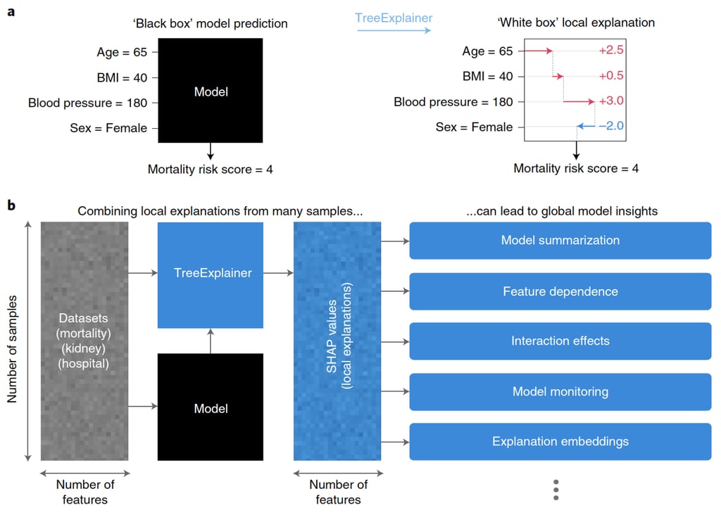
Local explanations provide a wide variety of new ways to understand global model structure — Image by Lundberg et al., 2020
This process for measuring local and global contributions to some goal can be related to DL using the method shown above and outlined in more detail in Lundberg et al., 2020. We can examine different combinations of model inputs (i.e. radar data subsets, or atmospheric variable combinations) to see how model accuracy changes. This can then be used to identify which variables, and which locations within the atmosphere in our case, provide the most important information for actively retrieving snowfall. Note that this is a very computationally expensive analysis to perform.
Breaking our dataset into different intensity precipitation event types and performing a Shapley analysis on each subset reveals the most important variables and regions (below; darker shaded regions indicate higher importance).
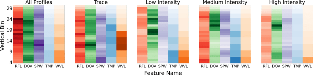
Heatmap of Shapley values for each model predictor for each vertical bin above the surface — Image by Author
Interestingly, and perhaps unexpectedly, we find that DeepPrecip values areas in the mid-upper region of the atmosphere (near 2 km) as the most important contributors. Not just near surface bins. Typically, radar-based snowfall retrievals rely on information from a single (or handful) of near-surface bins, but that does not appear the be the case here. Additionally, reflectivity (RFL) is usually considered as the most important variable in radar-based retrievals, however Doppler Velocity (DOV) actually surpasses RLF in important for high intensity precipitation events. Note that SPW is spectral width, TMP is temperature and WVL is wind velocity.
Understanding how our DL model is making decisions is an important step for further optimizing its performance and improving its skill in future iterations. Further, the information revealed in this analysis could help to inform current and future snowfall retrievals for next-generation precipitation missions. If you are performing a similar experiment with DL, I would highly recommend testing this process out on your own model as these outputs can be quite illuminating!
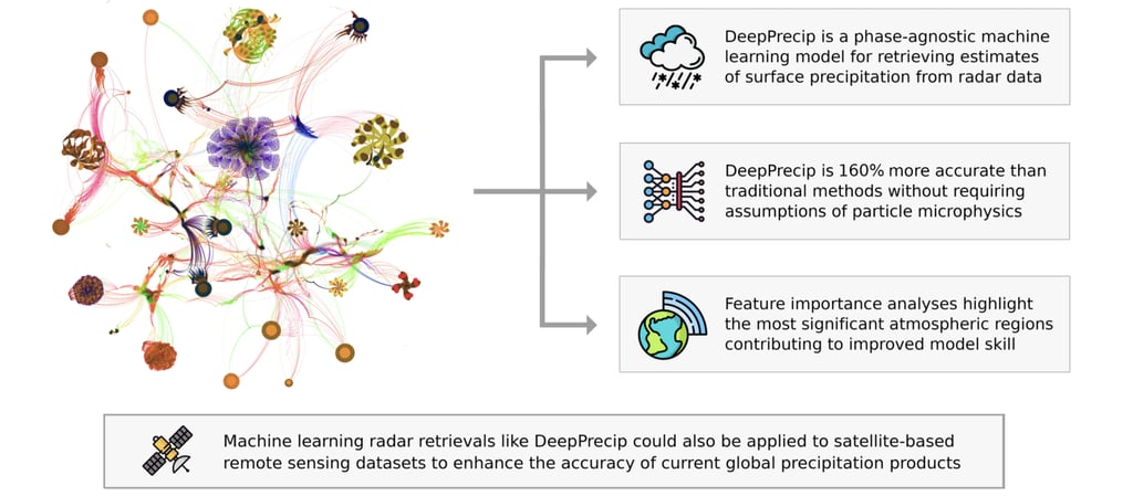
DeepPrecip project summary and next steps — Image by Author
In this work, we briefly describe the development process of DeepPrecip: a novel deep learning snowfall retrieval algorithm using vertical reflectivity profiles. While we don’t discuss the code for DeepPrecip here, the model is open source and available for use on GitHub. It was developed in Python using scikit-learn, Tensorflow and Keras.
If you are interested in testing things out, the model can be built and run using the following commands:
git clone https://github.com/frasertheking/DeepPrecip.git

conda env create -f req.yml

conda activate deep_precip

python deep_precip.py
We also include a deep_precip_ipu.py module for running this model on Graphcore IPUs. Note that you will need MRR training data to feed as an input to the model.
I’ll conclude this post by saying that I don’t expect DL models to completely replace physical models or traditional empirical methods for snowfall retrievals. However, the high accuracy and robustness of a DL approach, combined with the insights provided from global model behaviour analyses can help to enhance and inform future snowfall retrieval methods for both surface and spaceborne radar missions.
For more specifics on this project, please read our paper currently in review at Atmospheric Measurement Techniques (AMT).
Further, if you’d like to support our work, we are finalists in the NSERC Science Exposed contest, and would appreciate your support by voting for our image.
I’d like to thank the many data providers who contributed years of observations to this work, my coauthors, the University of Waterloo as well as the Graphcore team for their continued support and access to their computing systems.
I would also like to thank the Natural Sciences and Engineering Research Council of Canada (NSERC) for funding this project.
Ashouri, Hamed, Gehne, Maria & National Center for Atmospheric Research Staff (Eds). Last modified 31 Oct 2021. “The Climate Data Guide: PERSIANN-CDR: Precipitation Estimation from Remotely Sensed Information using Artificial Neural Networks — Climate Data Record.”
Dramsch, J. S. (2020). 70 years of machine learning in geoscience in review. Advances in Geophysics, 61, 1–55. https://www.sciencedirect.com/science/article/pii/S0065268720300054
Gray, D. M. ed, & Male, D. H. ed. (1981). Handbook of snow: Principles, processes, management & use. Pergamon Press. https://snia.mop.gob.cl/repositoriodga/handle/20.500.13000/2981
IPCC, 2019: IPCC Special Report on the Ocean and Cryosphere in a Changing Climate [H.-O. Pörtner, D.C. Roberts, V. Masson-Delmotte, P. Zhai, M. Tignor, E. Poloczanska, K. Mintenbeck, A. Alegría, M. Nicolai, A. Okem, J. Petzold, B. Rama, N.M. Weyer (eds.)]. Cambridge University Press, Cambridge, UK and New York, NY, USA, 755 pp. https://doi.org/10.1017/9781009157964.
King, F., Duffy, G., & Fletcher, C. G. (2022). A Centimeter Wavelength Snowfall Retrieval Algorithm Using Machine Learning. Journal of Applied Meteorology and Climatology, 1(aop). https://doi.org/10.1175/JAMC-D-22-0036.1
King, F., Duffy, G., Milani, L., Fletcher, C. G., Pettersen, C., & Ebell, K. (2022). DeepPrecip: A deep neural network for precipitation retrievals. EGUsphere, 1–24. https://doi.org/10.5194/egusphere-2022-497
Krumbein, W. C., & Dacey, M. F. (1969). Markov chains and embedded Markov chains in geology. Journal of the International Association for Mathematical Geology, 1(1), 79–96. https://doi.org/10.1007/BF02047072
Li, L., Jamieson, K., DeSalvo, G., Rostamizadeh, A., & Talwalkar, A. (2018). Hyperband: A Novel Bandit-Based Approach to Hyperparameter Optimization (arXiv:1603.06560). arXiv. https://doi.org/10.48550/arXiv.1603.06560
Lundberg, S. M., Erion, G., Chen, H., DeGrave, A., Prutkin, J. M., Nair, B., Katz, R., Himmelfarb, J., Bansal, N., & Lee, S.-I. (2020). From local explanations to global understanding with explainable AI for trees. Nature Machine Intelligence, 2(1), 56–67. https://doi.org/10.1038/s42256-019-0138-9
Musselman, K. N., Addor, N., Vano, J. A., & Molotch, N. P. (2021). Winter melt trends portend widespread declines in snow water resources. Nature Climate Change, 11(5), 418–424. https://doi.org/10.1038/s41558-021-01014-9
Newendorp, P. D. (1976). Decision analysis for petroleum exploration. https://www.osti.gov/biblio/6406439
Preston, Floyd W., and James Henderson. Fourier series characterization of cyclic sediments for stratigraphic correlation. Kansas Geological Survey, 1964.
Stephens, G. L., 1994: Remote Sensing of the Lower Atmosphere: An Introduction. Oxford University Press, 562 pp.
Sturm, M., Goldstein, M. A., & Parr, C. (2017). Water and life from snow: A trillion dollar science question. Water Resources Research, 53(5), 3534–3544. https://doi.org/10.1002/2017WR020840
>Talaat, F. M., & Gamel, S. A. (2022). RL based hyper-parameters optimization algorithm (ROA) for convolutional neural network. Journal of Ambient Intelligence and Humanized Computing. https://doi.org/10.1007/s12652-022-03788-y
Wood, N. B., L’Ecuyer, T. S., Heymsfield, A. J., Stephens, G. L., Hudak, D. R., & Rodriguez, P. (2014). Estimating snow microphysical properties using collocated multisensor observations. Journal of Geophysical Research: Atmospheres, 119(14), 8941–8961. https://doi.org/10.1002/2013JD021303
Thanks to Alyssa Francavilla and Katherine Prairie
Share: