Getting started with PyTorch Geometric (PyG) on Graphcore IPUs

Graphcore IPUs can significantly accelerate both the training and inference of Graph Neural Networks (GNNs).

With the latest Poplar SDK 3.2 from Graphcore, using PyTorch Geometric (PyG) on IPUs for your GNN workloads has never been easier.

Using a set of tools based on PyTorch Geometric, which we have packaged as PopTorch Geometric, you can start accelerating your GNN model on IPUs in no time. 

In this blog we will show how to easily get started with PyG on IPUs. We will go through an end-to-end example that accelerates training on IPUs, with a few tips and tricks to familiarise yourself with PyG usage on IPUs. And finally, we will introduce PopTorch Geometric data loaders which will enable you to get the most out of the IPU for your GNN workloads.

We also encourage you to check out our blog Accelerating PyG on IPUs: unleash the power of Graph Neural Networks to discover more about how and why IPUs are a great fit for your GNNs workloads . 

You can get started for free straight away on Paperspace, either by exploring a range of introductory tutorials, some more in-depth application examples or benchmarks demonstrating the great performance of IPUs on message passing operations.

Porting to the IPU: basics

To run your workload using PyTorch Geometric on IPUs, the model will need to target PopTorch. PopTorch is a set of IPU-specific extensions allowing you to run PyTorch native models on the IPU. It is designed to require as few changes as possible from native PyTorch, but there are some differences to be aware of: we will explore them in the rest of this section.   

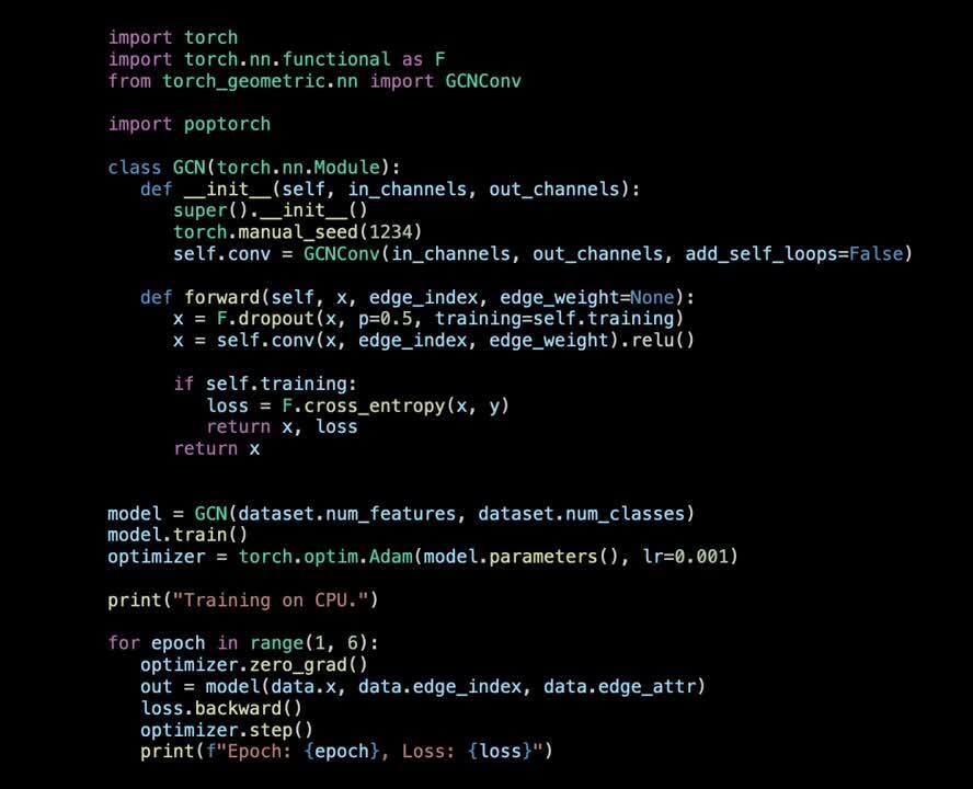
Let's start from a typical model using PyG: 

import torch
import torch.nn.functional as F
from torch_geometric.nn import GCNConv

class GCN(torch.nn.Module):
    def __init__(self, in_channels, out_channels):
        super().__init__()
        torch.manual_seed(1234)
        self.conv = GCNConv(in_channels, out_channels, add_self_loops=False)

    def forward(self, x, edge_index, edge_weight=None):
        x = F.dropout(x, p=0.5, training=self.training)
        x = self.conv(x, edge_index, edge_weight).relu()
        return x


model = GCN(dataset.num_features, dataset.num_classes)
model.train()
optimizer = torch.optim.Adam(model.parameters(), lr=0.001)

print("Training on CPU.")

for epoch in range(1, 6):
    optimizer.zero_grad()
    out = model(data.x, data.edge_index, data.edge_attr)
    loss = F.cross_entropy(out, data.y)
    loss.backward()
    optimizer.step()
    print(f"Epoch: {epoch}, Loss: {loss}")

The concepts in the above block of code are probably already familiar to you. We have created a simple model comprising of a single GCNConv layer imported from PyG, selected an optimizer and constructed a training loop where we calculate the loss and do the optimizer update. 

Now let's implement the minimal changes to get this model ready for running on IPUs:  

In the video above, after importing PopTorch, we have:

•  Moved the loss function inside the forward method of your model.
• Wrapped the model in poptorch.trainingModel as we intend to run training in this snippet. We would have wrapped it using poptorch.inferenceModel if we intended instead to run inference.
• Used a PopTorch optimizer, specifically designed for the IPU.
• Removed the manual call to the backward pass and optimizer steps - both are handled by PopTorch automatically.

import torch
import torch.nn.functional as F
from torch_geometric.nn import GCNConv

import poptorch

class GCN(torch.nn.Module):
    def __init__(self, in_channels, out_channels):
        super().__init__()
        torch.manual_seed(1234)
        self.conv = GCNConv(in_channels, out_channels, add_self_loops=False)

    def forward(self, x, edge_index, y, edge_weight=None):
        x = F.dropout(x, p=0.5, training=self.training)
        x = self.conv(x, edge_index, edge_weight).relu()

        if self.training:
            loss = F.cross_entropy(x, y)
            return x, loss
        return x


model = GCN(dataset.num_features, dataset.num_classes)
model.train()
optimizer = poptorch.optim.Adam(model.parameters(), lr=0.001)
poptorch_model = poptorch.trainingModel(model, optimizer=optimizer)

print("Training on IPU.")

for epoch in range(1, 6):
    output, loss = poptorch_model(
        data.x, data.edge_index, data.y, edge_weight=data.edge_attr
    )
    print(f"Epoch: {epoch}, Loss: {loss}")

And voilà! With those simple changes you can successfully run your PyG model on IPUs. We are now ready to go more in depth using an end-to-end example.

End-to-end example: simple GCN based GNN for node classification

Let's apply the concepts we described above in an example where we will classify the nodes of the Cora dataset using a simple model, made up of a couple of GCN layers. The Cora dataset is a citation network where a node represents a document, and an edge exists if there is a citation between the two documents. 

First, let’s load the dataset: 

from torch_geometric.datasets import Planetoid
import torch_geometric.transforms as T

transform = T.Compose([T.NormalizeFeatures(), T.AddSelfLoops()])

dataset = Planetoid(root=dataset_directory, name="Cora", transform=transform)
data = dataset[0]  # Access the citation graph as Data object

PyG provides a lot of useful layers that allow you to build GNNs in only a few lines of code. For this task we will use the GCNConv layer, as GCN is one of the most used GNN operators. 

Before we define the model, we should first understand that PyTorch support on the IPU relies on ahead-of-time compilation via PopTorch. The compiler performs static analysis of the computational graph: prior knowledge of the input tensors shapes is required to optimise the evaluation on the IPU. Many of the changes we will make in this example and beyond are driven by ensuring the model can be successfully compiled. 

We are now ready to define the model with a few observations in mind:

•  GCNConv self-loops are disabled. This is because we have added the self-loops to the dataset as a transform when loading the dataset as per the code snippet above, hence we can turn them off in the layer. This change is also required to ensure our compiled graph for the IPU is static.
• PopTorch requires the loss function to be part of the model, so we will move it inside the forward method.
• We will set the labels of the non-training nodes to -100 so that they are ignored in the loss function: this step uses torch.where() which ensures y is a known size, satisfying the requirement of static size inputs on IPUs.  

import torch
from torch_geometric.nn import GCNConv
import torch.nn.functional as F


class GCN(torch.nn.Module):
    def __init__(self, in_channels: int, out_channels: int):
        super(GCN, self).__init__()
        self.conv1 = GCNConv(in_channels, 16, add_self_loops=False)
        self.conv2 = GCNConv(16, out_channels, add_self_loops=False)

    def forward(self, x, edge_index, y=None, train_mask=None):
        x = self.conv1(x, edge_index).relu()
        x = F.dropout(x, training=self.training)
        x = self.conv2(x, edge_index).relu()
        x = F.log_softmax(x, dim=1)

        if self.training:
            y = torch.where(train_mask, y, -100)
            loss = F.nll_loss(x, y)
            return x, loss
        return x

We will then wrap the model in a PopTorch trainingModel() and we will use a PopTorch optimizer (Adam in this case). Using a PopTorch specific optimizer can help improve speed and memory utilisation: those are very straightforward to use as they are drop-in replacements for existing PyTorch optimizers.

model = GCN()
model.train()
optimizer = poptorch.optim.Adam(model.parameters(), lr=0.001)
poptorch_model = poptorch.trainingModel(model, optimizer=optimizer)

Now we can run the training and make sure that the loss decreases nicely: 

for epoch in range(1, 101):
    out, loss = poptorch_model(
        data.x, data.edge_index, y=data.y, edge_weight=data.edge_attr, train_mask=data.train_mask
    )
    print(f"Epoch: {epoch}, Loss: {loss}")

And that’s all there is to do to train our model on IPUs! Next step is to take a look at inference.

Running inference

To run inference in PopTorch we will take our trained model, set it to eval mode and wrap it in a PopTorch inferenceModel(). 

model.eval()
poptorch_inf_model = poptorch.inferenceModel(model)

As we are not training anymore, we don't need a loss to be defined so we can get away with not doing any masking in the model itself. Instead, we can do the masking afterwards on the CPU. First, we get the predictions from the model: 

data = next(iter(dataset))
logits = poptorch_inf_model(data.x, data.edge_index)
pred = logits.argmax(dim=1)

Now we can calculate the validation accuracy on the CPU. This is ok as these are relatively inexpensive operations, however there is nothing stopping us from putting these in our model definition and having them computed on the IPU instead. 

correct_results = pred[data.val_mask] == data.y[data.val_mask]
accuracy = int(correct_results.sum()) / int(data.val_mask.sum())
print(f"Validation accuracy: {accuracy:.2%}")

And with that we have obtained a validation accuracy for our trained model. 

This was a very simple example where we were able to do full batch updates, i.e. we could process the full graph in a single batch. As the input graph size increases, this may not always be the case. In the next session we will show use cases where full batch updates are not possible or may not be desirable: here is when dataloading comes into play. Let’s find out how to make the most of dataloaders on IPUs.  

Utilising PopTorch Geometric's high performance data loaders 

One key part of any model in training and inference is preparing your data, batching and feeding it into your model. 

If you’re working with GNNs, your input data might be a set of small graphs that you can batch together or a larger graph requiring either sampling or full batch update. 

In the previous section we highlighted how the IPU needs fixed sized inputs, which means that prior knowledge of the shape of the input tensors is required. There are different ways to achieve this, and the method used will depend on the type of input graph dataset we're working with:

• If we're dealing with a dataset of many small graphs, we can batch the input graphs via the dataloader and pad the resulting batch. With our latest tools provided in PopTorch Geometric this is very simple to achieve using the FixedSizeDataLoader. You can check out our tutorial on Small Graph Batching with Padding for a detailed walkthrough. This approach may result in a very large amount of padding in specific use cases: we present a more efficient batching strategy called packing in a dedicated tutorial on Small Graph Batching with Packing.
• If we're dealing with a dataset of a single large graph, we can sample from it and then pad the samples to obtain static shapes. In PopTorch Geometric we provide a tool to produce fixed size clusters ready to be used for your large graph workload, the FixedSizeClusterLoader. You can refer to the Cluster CGN example for a large graph use case of this. 
• If your graph is of medium size where a full batch update is possible then the fixed size requirement becomes trivial, as there is only a single batch each batch will be the same size. We saw this simple case in the end-to-end example above.

Using any of the data loaders provided in PopTorch Geometric, like those mentioned above, also unlocks some features that can help accelerate your model, for example:

• Enabling replication to parallelise your model across multiple IPUs.
• Turning up the number of iterations the IPU computes before returning to the host.
• Enabling gradient accumulation to unlock features such as pipelining, allowing larger models to be distributed over multiple IPUs.
• Enabling asynchronous data loading. 

Conclusion 

We have seen how simple it is to start using IPUs for your GNN workload with PyTorch Geometric by leveraging tools to accelerate your dataloading and get the most out of the IPU. For a more in-depth overview about the competitive advantage IPUs offer when working with GNNs, read Accelerating PyG on IPUs: unleash the power of Graph Neural Networks.

You can get started today for free on Paperspace with our PyG specific runtime: it has everything ready for you to start accelerating your PyG model on IPUs.