BERT-Large Training on the IPU explained

BERT is one of today’s most widely used natural language processing models, thanks to its accuracy and flexibility. It is also one of the most highly requested models by Graphcore customers. 

Our engineers have implemented and optimized BERT for our IPU systems to support a huge range of language-based applications, demonstrating excellent throughput using industry-standard machine learning training schemes. 

Here, we will explain in detail the optimization techniques engineers from Graphcore’s Applications, Software and China Engineering teams have used to pre-train and fine-tune our BERT-Large implementation.

The rise of BERT

Bidirectional Encoder Representations from Transformers (BERT) is a transformer-based language representation model created by Google. It has seen dramatic growth in popularity since it was released in late 2018.

Initially trialled on around 10% of Google's US English-language search queries, BERT is today used for almost every English-language Google search. 

As well as search engines, BERT and its derivatives have been applied to other domains such as question answering, content-based recommendation, video understanding and protein feature extraction, demonstrating its versatility.

Unlike previous transformer models, such as the Generative Pre-trained Transformer (GPT), BERT was designed to take advantage of the left and right context of each unlabelled training example in all transformer layers and effectively retrieve its representations in both directions. This bidirectional attention gives greater flexibility for a wide variety of downstream tasks.

BERT’s ability to use a huge, unlabelled dataset in the pre-training phase (and achieve state-of-the-art accuracy in the fine-tuning phase with just a small amount of labelled data) makes large, BERT-like transformer-based language models very attractive. Because of this, the demand for training and fine-tuning these large neural-network language models is growing dramatically.

As well as large-scale tasks such as language modelling, very small-scale downstream tasks can also benefit from these approaches. For example, the Microsoft Research Paraphrase Corpus (MRPC) only has 3600 training samples, but the accuracy is improved from 84.4 to 86.6% by increasing the model size from BERT-Base to BERT-Large. BERT variants retain the lead over MRPC and many similar benchmarks. 

As machine learning researchers and engineers look to continue improving the task performance of these models, model sizes are getting bigger and bigger. This can be seen both within the BERT model variants and several other more recent models, such as GPT-3 with its 175 billion parameters.

Pre-training BERT on the IPU-POD

It’s not only advances in modelling that make this possible. Developing new AI hardware and systems that can offer better efficiency will also enable us to train these large-scale models within a reasonable timeframe, potentially pre-training billions of samples in days or even hours. Graphcore’s IPU‑POD system addresses this performance challenge and greatly increases productivity for researchers and engineers. The IPU-POD system leverages extremely high-performance In-Processor Memory to deliver excellent computational performance and better power efficiency by minimizing data movement. High-speed scale-out interconnect and intelligent memory management enable applications to scale efficiently to hundreds of IPUs. 

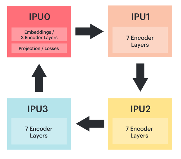
To run BERT efficiently on the IPU‑POD, we load the entire model’s parameters onto the IPUs. To do this, we split, or “shard”, the BERT model across four IPUs and execute the model as a pipeline during the training process.

Below you can see an example of how we partition BERT-Large. IPU 0 contains the embedding layer and projection/loss layers along with three encoder layers and the remaining 21 layers are evenly distributed over the other three IPUs. Since the embedding and projection layers share parameters, we can place the projection, masked language model (MLM) and next sentence prediction (NSP) layers back on IPU 0.

To help reduce the memory footprint on-chip, we use recomputation. This means we don’t have to store intermediate layer activations for use when calculating the backward passes. Recomputation is a strategy which can be employed when training models, and it is particularly useful when implementing a pipelining strategy. As we have multiple batches “in-flight” through the pipeline at any time, the size of stored activations can be significant if we don’t use recomputation.

The optimizer state for the pre-training system is stored in Streaming Memory and loaded on demand during the optimizer step. 

Streaming Memory is how we describe memory off chip at Graphcore. Each of the core “building block” IPU-M2000 platforms within an IPU-POD₆₄ system has up to 450GB of memory which can be addressed by its 4 IPUs. This is divided up into the 900MB of In-Processor Memory included in every IPU chip and up to 112GB per IPU of off-chip Streaming Memory. This Streaming Memory is supported by DDR4 DIMMs on the IPU-Machine.

Graphcore’s BERT Implementation in TensorFlow, PyTorch & PopART

In Graphcore examples on our GitHub Application Examples, you can find implementations of BERT for the IPU in TensorFlow, PyTorch and PopART. 

Our TensorFlow implementation shares model code with the original Google BERT implementation, with customization and extension to leverage Graphcore’s TensorFlow pipelining APIs.

Our PyTorch implementation is based on model descriptions and utilities from the Hugging Face transformers library. We use the Graphcore PopTorch library to target the IPU, including pipelined execution, recomputation and multi-replica/data parallelism.

A BERT implementation using the Poplar Advanced Runtime (PopART) is also available on our Github. PopART enables you to import or create models from an ONNX model description for both training and inference, and includes both a C++ API and a Python API. PopART supports optimizer, gradient and parameter partitioning as described in this paper. We collectively describe these as replicated tensor sharding (RTS). For our replicated pipeline model-parallel BERT system in PopART, we use optimizer and gradient partitioning.

Scaling BERT to the IPU-POD

Unsupervised pre-training enables BERT to take advantage of the billions of training samples in Wikipedia, BookCorpus and other sources. Even with the IPU‑POD₄, multiple passes over these large datasets take a significant amount of time. To reduce training time, we use data-parallel model training to scale the pre-training process to IPU‑POD₁₆, IPU‑POD₆₄ and beyond.

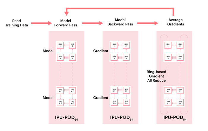
Data-parallel training involves breaking the training dataset up into multiple parts, which are each consumed by a model replica. At each optimization step, the gradients are mean-reduced across all replicas so that the weight update and model state are the same across all replicas.

Collective gradient reduction

The gradient reduction uses the Graphcore Communication Library (GCL), an extension to our Poplar software stack designed to enable high-performance scale-out. GCL includes a highly efficient ring-based All-Reduce, along with many other common communication primitives.  Gradients are averaged across all replicas as illustrated in the image below, and weight updates are applied once all multi-replica gradients are fully reduced.

Data-parallel gradient reduction can be added automatically using optimizer wrapper functions, or with finer control in custom optimizer definitions. This reduction can happen seamlessly within an IPU-POD or between different IPU-PODs.

For more details on how the API works in TensorFlow, you can read about Replicated Graphs in the TensorFlow user guide.

For PyTorch, we set a replication factor in the PopTorch IPU model options.

Training BERT with large batches

One of the main contributors to the parallel scaling efficiency of the model is how frequently the gradients need to be communicated. We use Gradient Accumulation (GA) to decouple the compute or micro-batch size from the global batch size. This also enables us to maintain a constant global batch size when varying the number of IPUs and/or replicas by adjusting the gradient accumulation factor: global batch size = replica batch size × number of replicas, where replica batch size = compute batch size × gradient accumulation factor.

For a fixed number of replicas, a larger global batch size therefore enables a higher GA factor and fewer optimizer and communication steps.

However, if the GA is too large, such as several thousand, this can cause underflow problems with FP16. In the case of a small GA, this can lead to low pipeline efficiency due to the bubble overhead, as described here. Some experimentation may be required to find the optimal value.

In the following sections, we will review learning rate, warmup and optimizer schemes we leverage when training BERT.

Linear scaling rule

In this paper on training ImageNet with SGD minibatches, the researchers used a linear scaling rule when training large global batches for ResNet-50 and Mask R-CNN. This rule determines that when the replica batch size \(n\) is multiplied by \(k\), (where \(k\) is usually the number of model replicas), the base learning rate, \(\eta\), should be multiplied by \(k\) and set to \(k \eta\).

Increasing global batch sizes from \(n\) to \(n k\), while using the same number of training epochs and maintaining the testing accuracy, can reduce the total training time by a factor of \(k\) and dramatically shorten the model-to-production time. However, task performance is shown to degrade with large global batches.

Gradual warmup strategy

One way of mitigating this is warmup, where the learning rate is not initialized as \(k \eta\) immediately. Instead, the training procedure starts with a zero, or arbitrary small, learning rate and linearly increases it over a predefined number of warmup steps until it reaches \(k \eta\). This gradual warmup enables large global batch training with many fewer steps to achieve similar training accuracy to the smaller batch size. In the training ImageNet with SGD minibatches paper, this enabled training with a global batch size of ~8,000.

The predefined warmup steps are different for phase 1 and phase 2 in the BERT-Large pre-training case. As in the BERT paper, our phase 1 uses training data with a maximum sequence length of 128, and a maximum sequence length of 384 for phase 2. The warmup for phase 1 is 2000 steps, which accounts for around 30% of the entire training steps in phase 1. In comparison, during phase 2 there are 2100 steps in total, and approximately 13% of these steps are warmup.

The warmup steps may need to be tuned for different pre-training datasets.

AdamW optimizer

The standard stochastic gradient descent algorithm uses a single learning rate for all weight updates and keeps it constant during training. In contrast, Adam (adaptive moment estimation) makes use of the moving exponential average of the first and second moments of gradients, and adapts the learning-rate parameter based on these moments.

In their ICLR 2019 paper, researchers Loshchilov and Hutter discovered that L2 regularization is not effective in Adam. Instead, they proposed AdamW which applies weight decay regularization during the weight update step instead of L2 regularization at the loss function. This allows weights to decay multiplicatively rather than by an additive constant factor. They demonstrated that AdamW with warm restarts has better training loss and generalization error for both CIFAR-10 and ResNet32x32.

In IPU‑POD₁₆ BERT pre-training, we experimented with AdamW using pre-training global batch sizes ranging from 512 to 2560, all achieving convergence to reference accuracy when fine-tuned on the SQuAD downstream task.

LAMB optimizer

The LAMB optimizer (described in more detail here) is designed to overcome gradient instability and loss divergence caused by growing the batch size, enabling even larger batch sizes. LAMB uses the same layer-wise normalization concept as layer-wise adaptive rate scaling (LARS) so the learning rate is layer sensitive. However, for the parameter updates it uses the momentum and variance concept from AdamW instead.

The learning rate for each layer is calculated by:

\[\eta \frac{ \| x \| } { \| g \| }\]

where \(\eta\) is the overall learning rate, \(\| x \|\) is the norm of the parameters of this layer, and \(\| g \|\) is norm of the updates for the same AdamW optimizer.

This means LAMB normalizes the update and then multiplies it by \(\|x\|\) so that it will be of the same order of magnitude as the parameters of each layer, ensuring that the update makes some real change to each layer. Then the result is multiplied by the overall learning rate \(\eta\).

In LAMB, the weights and biases are considered as two separate layers because both have very different trust values and therefore should be treated with different learning rates. Biases and gamma, beta of batch-norm or group-norm are often excluded from layer adaption.

For BERT, LAMB enables global batch sizes of up to 65,536 in phase 1 and up to 32,768 in phase 2.

Low-precision training

During the early evolution of deep learning, many models were trained using 32-bit precision floating-point arithmetic. Using lower precision is attractive because it enables both higher computational throughput – for IPUs, FP16 peak performance is four times higher than FP32. With lower precision, the size of tensors is reduced by a factor of two, lowering memory pressure and communication costs.

However, FP16 precision floating point has both lower precision and lower dynamic range than FP32. Others have proposed using FP16 for the calculation of the forward pass (activations) and backward pass (gradients) using loss scaling to manage the dynamic range of the activations and gradients, while retaining an FP32 copy of the master weights with FP32 accumulation of the weight gradients.

We implement loss scaling in a similar fashion when training with activations and gradients in FP16.

Graphcore IPUs have the capability to use stochastic rounding, as well as traditional IEEE rounding modes. Stochastic rounding is based on a probability that is proportional to the proximity of a value to the upper and lower rounding bounds. Over a large number of samples this produces an unbiased rounding result.

Using stochastic rounding allows us to keep our weights in FP16 throughout the training process with no perceptible loss of accuracy in the end-to-end training or downstream task performance.

The first and second order moments in the optimizer are calculated and stored in FP32, and normalization is also carried out in FP32. The rest of the operations in the training process are calculated in FP16.

Training results

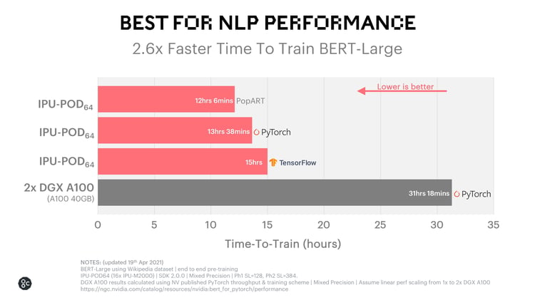
Graphcore’s latest scale-out system shows unprecedented efficiency for training BERT-Large, with up to 2.6x faster time to train vs a comparable DGX A100 based system. 

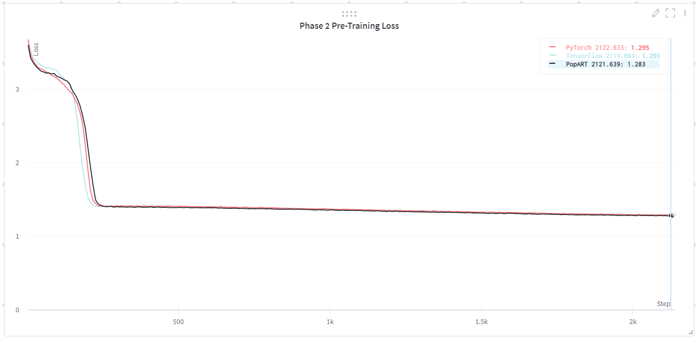
Containing 16 of our latest IPU-M2000 accelerators, the IPU-POD₆₄ draws on innovations in compute, communication and memory technologies to deliver the same accuracy as leading AI platforms on BERT-Large in a much shorter timeframe. In the chart below we provide results using the standard high-level frameworks of TensorFlow and PyTorch, along with our own PopART based implementation. These are compared against NVIDIA’s best published results which were for PyTorch and using a similar methodology to derive a comparable time-to-train result. 

Pre-training accuracy

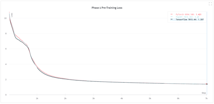
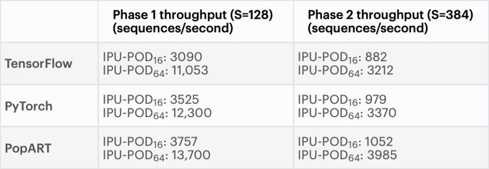
The charts below show the pre-training loss curves for our TensorFlow, PyTorch and PopART implementations, showing convergence to equivalent final training loss and very similar training curves. We also include training throughputs for all three model implementations on IPU-POD₁₆  and IPU-POD_64.

Table: Pre-training throughput

Fine-tuning accuracy

After we have sufficiently trained BERT, which may need hundreds of millions of training samples, we can use these pre-trained weights as initial weights for a task-specific fine-tuning training process with a smaller amount of labelled data.

This two-phase setup is widely used in practice because it offers the following advantages:

• We only need to pre-train the BERT model once, for all fine-tuning tasks
• Fine-tuning these pre-trained models delivers good task performance with less labelled data, saving a lot of human effort to label task-specific data

Fine-tuning can be completed in minutes or hours on an IPU‑POD₄ or IPU‑POD₁₆, depending on the size of the training dataset. Many fine-tuning trainings can be stopped after a small number of passes over the training sets.

SQuAD v1.1

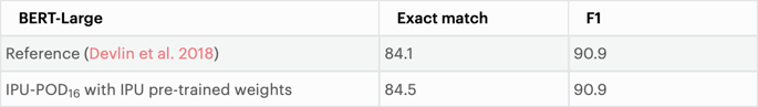
The Stanford Question Answering Dataset (SQuAD) v1.1 is a large reading comprehension dataset which contains more than 100,000 question-answer pairs in 500+ articles. 

The table below shows the accuracy when we fine-tune BERT-Large with the SQuAD v1.1 task on IPUs using reference pre-trained and IPU pre-trained weights. As demonstrated, IPUs can exceed reference accuracy for this task. 

Table: SQuAD 1.1 task accuracy on the IPU

CLUE

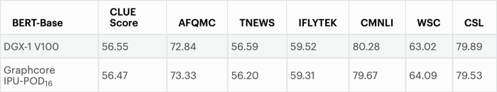
The next set of data we will look at shows the accuracy when we fine-tune BERT-Base with Chinese Language Understanding Evaluation (CLUE) tasks on IPUs, using Google pre-trained weights. 

The CLUE score is the average of the test accuracy over all the CLUE tasks. Each task’s test accuracy is the average of five experiment results. As shown in the table below, IPUs can achieve the same accuracy as other AI platforms such as DGX-1 V100.

Table: CLUE task accuracy on GPU and IPU

With just a few optimizations, AI practitioners can use IPU-POD systems to significantly reduce training time for BERT-Large without compromising on accuracy. As we’ve seen, it is much more straightforward than you might think to run a large model like BERT on our new hardware architecture. You will probably be familiar with many of the optimization techniques we have described here. We have also made our TensorFlow and PyTorch implementations available, so that any machine learning practitioner can take a look at how they would use these frameworks to run BERT on the IPU. 

As researchers and engineers are increasingly looking to larger models such as BERT to achieve the best possible task performance, hardware efficiency is going to play a critical role. Here, we have seen that by using IPU-POD systems, innovators can not only reap the accuracy advantages of BERT-Large and similar models but also benefit from significant performance gains. The unique characteristics of IPU processor architecture make it possible to accelerate today’s most advanced models while allowing us to reimagine how tomorrow’s state-of-the-art models should be developed, all in a familiar software environment. 

Thank you to our engineers who led this work:

James Briggs, Oskar Bunyan, Lorenzo Cevolani, Arjun Chandra, Nic Couronneau, Lakshmi Krishnan, Guoying Li, Visu Loganathan, Sam Maddrell-Mander, Zhiwei Tian, Sylvain Viguier, Xian Wang, Xihuai Wen, ChengShun Xia, Han Zhao

In addition to the names above, thank you to the BERT applications, PopART, TensorFlow, PyTorch, GCL and Poplar teams at Graphcore for their support with implementing and optimizing BERT for IPU systems.